
CDA学习之Pandas - 十分钟搞定Pandas / Pandas秘籍
发布于2021-07-25 07:05 阅读(1534) 评论(0) 点赞(14) 收藏(4)
前言
这篇博文是根据Pandas 官方教程PDF文件整理而来,原文是PDF格式,没法直接复制到页面上来,所以我边看,边做,边整理到这来。
主要内容和数据保持了原文的原貌,特别保留了原文的链接,所以文章内容的版权归原文作者,我只是从PDF中搬出来,方便学习和查阅。
官方教程是官方文档的教程页面上的教程。
| 名称 | 原文 | 译者 |
|---|---|---|
| 十分钟搞定 pandas | 10 Minutes to pandas | ChaoSimple |
| Pandas 秘籍 | Pandas cookbook | 飞龙 |
| 学习 Pandas | Learn Pandas | 派兰数据 |
快速入门:十分钟搞定 Pandas
原文:10 Minutes to pandas
译者:ChaoSimple
来源:【原】十分钟搞定pandas
官方网站上《10 Minutes to pandas》的一个简单的翻译,原文在这里。这篇文章 是对 pandas 的一个简单的介绍,详细的介绍请参考:秘籍 。习惯上,我们会按下 面格式引入所需要的包:
In [1]: import pandas as pd
In [2]: import numpy as np
In [3]: import matplotlib.pyplot as plt
0.1 创建对象
可以通过 数据结构入门 来查看有关该节内容的详细信息。
1、可以通过传递一个 list 对象来创建一个 Series ,pandas 会默认创建整型 索引:
In [4]: s = pd.Series([1,3,5,np.nan,6,8])
In [5]: s
Out[5]:
0 1.0
1 3.0
2 5.0
3 NaN
4 6.0
5 8.0
dtype: float64 3
2、通过传递一个 numpy array ,时间索引以及列标签来创建一 个 DataFrame :
 In [6]: dates = pd.date_range('20130101', periods=6)
 In [7]: dates
 Out[7]:
 DatetimeIndex(['2013-01-01', '2013-01-02', '2013-01-03', '2013-0 1-04', '2013-01-05', '2013-01-06'], dtype='datetime64[ns]', freq='D')
 In [8]: df = pd.DataFrame(np.random.randn(6,4), index=dates, columns=list('ABCD'))
 In [9]: df
 Out[9]:
 				A 		B 		C 		D
 2013-01-01 0.469112 -0.282863 -1.509059 -1.135632
 2013-01-02 1.212112 -0.173215 0.119209 -1.044236
 2013-01-03 -0.861849 -2.104569 -0.494929 1.071804
 2013-01-04 0.721555 -0.706771 -1.039575 0.271860
 2013-01-05 -0.424972 0.567020 0.276232 -1.087401
 2013-01-06 -0.673690 0.113648 -1.478427 0.524988
3、通过传递一个能够被转换成类似序列结构的字典对象来创建一 个 DataFrame :
 In [10]: df2 = pd.DataFrame({ 'A' : 1.,
 ....: 						'B' : pd.Timestamp('20130102'),
 ....: 						'C' : pd.Series(1,index=list(range( 4)),dtype='float32'),
 ....: 						'D' : np.array([3] * 4,dtype='int3 2'),
 ....: 						'E' : pd.Categorical(["test","trai n","test","train"]),
 ....: 						'F' : 'foo' })
 ....:
 In [11]: df2
 Out[11]:
 	A 		B 		C D 	E F
 0 1.0 2013-01-02 1.0 3 test foo
 1 1.0 2013-01-02 1.0 3 train foo
 2 1.0 2013-01-02 1.0 3 test foo
 3 1.0 2013-01-02 1.0 3 train foo
4、查看不同列的数据类型:
 In [12]: df2.dtypes
 Out[12]:
 A 			float64
 B 	datetime64[ns]
 C 			float32
 D 			int32
 E 			category
 F 			object
 dtype: object
5、如果你使用的是 IPython,使用 Tab 自动补全功能会自动识别所有的属性以及自 定义的列,下图中是所有能够被自动识别的属性的一个子集:
 In [13]: df2.<TAB>
 df2.A 						df2.boxplot
 df2.abs 					df2.C
 df2.add 					df2.clip
 df2.add_prefix 		df2.clip_lower
 df2.add_suffix 		df2.clip_upper
 df2.align 				df2.columns
 df2.all 					df2.combine
 df2.any 					df2.combineAdd
 df2.append 			df2.combine_first
 df2.apply 				df2.combineMult
 df2.applymap 		df2.compound
 df2.as_blocks 		df2.consolidate
 df2.asfreq 				df2.convert_objects
 df2.as_matrix 		df2.copy
 df2.astype 				df2.corr
 df2.at 						df2.corrwith
 df2.at_time 			df2.count
 df2.axes 				df2.cov
 df2.B 						df2.cummax
 df2.between_time 	df2.cummin
 df2.bfill 					df2.cumprod
 df2.blocks 				df2.cumsum
 df2.bool 					df2.D
0.2 查看数据
详情请参阅:基础。
1、 查看 DataFrame 中头部和尾部的行:
In [14]: df.head()
Out[14]:
A B C D
2013-01-01 0.469112 -0.282863 -1.509059 -1.135632
2013-01-02 1.212112 -0.173215 0.119209 -1.044236
2013-01-03 -0.861849 -2.104569 -0.494929 1.071804
2013-01-04 0.721555 -0.706771 -1.039575 0.271860
2013-01-05 -0.424972 0.567020 0.276232 -1.087401
In [15]: df.tail(3)
Out[15]:
A B C D
2013-01-04 0.721555 -0.706771 -1.039575 0.271860
2013-01-05 -0.424972 0.567020 0.276232 -1.087401
2013-01-06 -0.673690 0.113648 -1.478427 0.524988
2、 显示索引、列和底层的 numpy 数据:
In [16]: df.index
Out[16]:
DatetimeIndex(['2013-01-01', '2013-01-02', '2013-01-03', '2013-0 1-04', '2013-01-05', '2013-01-06'], dtype='datetime64[ns]', freq='D')
In [17]: df.columns
Out[17]:
Index([u'A', u'B', u'C', u'D'], dtype='object')
In [18]: df.values
Out[18]:
array([[ 0.4691, -0.2829, -1.5091, -1.1356],
[ 1.2121, -0.1732, 0.1192, -1.0442],
[-0.8618, -2.1046, -0.4949, 1.0718],
[ 0.7216, -0.7068, -1.0396, 0.2719],
[-0.425 , 0.567 , 0.2762, -1.0874],
[-0.6737, 0.1136, -1.4784, 0.525 ]])
3、 describe() 函数对于数据的快速统计汇总:
In [19]: df.describe()
Out[19]:
A B C D
count 6.000000 6.000000 6.000000 6.000000
mean 0.073711 -0.431125 -0.687758 -0.233103
std 0.843157 0.922818 0.779887 0.973118
min -0.861849 -2.104569 -1.509059 -1.135632
25% -0.611510 -0.600794 -1.368714 -1.076610
50% 0.022070 -0.228039 -0.767252 -0.386188
75% 0.658444 0.041933 -0.034326 0.461706
max 1.212112 0.567020 0.276232 1.071804
4、 对数据的转置:
In [20]: df.T
Out[20]:
2013-01-01 2013-01-02 2013-01-03 2013-01-04 2013-01-05 2 013-01-06
A 0.469112 1.212112 -0.861849 0.721555 -0.424972 -0.673690
B -0.282863 -0.173215 -2.104569 -0.706771 0.567020 0.113648
C -1.509059 0.119209 -0.494929 -1.039575 0.276232 -1.478427
D -1.135632 -1.044236 1.071804 0.271860 -1.087401 0.524988
5、 按轴进行排序
In [21]: df.sort_index(axis=1, ascending=False)
Out[21]:
				D 		C 		B 			A
2013-01-01 -1.135632 -1.509059 -0.282863 0.469112
2013-01-02 -1.044236 0.119209 -0.173215 1.212112
2013-01-03 1.071804 -0.494929 -2.104569 -0.861849
2013-01-04 0.271860 -1.039575 -0.706771 0.721555
2013-01-05 -1.087401 0.276232 0.567020 -0.424972
2013-01-06 0.524988 -1.478427 0.113648 -0.673690
6、 按值进行排序
In [22]: df.sort_values(by='B')
Out[22]:
				A 		B 		C 		D
2013-01-03 -0.861849 -2.104569 -0.494929 1.071804
2013-01-04 0.721555 -0.706771 -1.039575 0.271860
2013-01-01 0.469112 -0.282863 -1.509059 -1.135632
2013-01-02 1.212112 -0.173215 0.119209 -1.044236
2013-01-06 -0.673690 0.113648 -1.478427 0.524988
2013-01-05 -0.424972 0.567020 0.276232 -1.087401
0.3 选择
虽然标准的 Python/Numpy 的选择和设置表达式都能够直接派上用场,但是作为工程使用的代码,我们推荐使用经过优化的 pandas 数据访问方式: .at , .iat , .loc , .iloc 和 .ix 。详情请参阅索引和选取数据 和 多重索引/高级索引。
0.3.1 [ ]获取
1、 选择一个单独的列,这将会返回一个 Series ,等同于 df.A :
In [23]: df['A']
Out[23]:
2013-01-01 0.469112
2013-01-02 1.212112
2013-01-03 -0.861849
2013-01-04 0.721555
2013-01-05 -0.424972
2013-01-06 -0.673690
Freq: D, Name: A, dtype: float64
2、 通过 [] 进行选择,这将会对行进行切片
In [24]: df[0:3]
Out[24]:
				A 			B 		C 		D
2013-01-01 0.469112 -0.282863 -1.509059 -1.135632
2013-01-02 1.212112 -0.173215 0.119209 -1.044236
2013-01-03 -0.861849 -2.104569 -0.494929 1.071804

In [25]: df['20130102':'20130104']
Out[25]:
				A 			B 		C 		D
2013-01-02 1.212112 -0.173215 0.119209 -1.044236
2013-01-03 -0.861849 -2.104569 -0.494929 1.071804
2013-01-04 0.721555 -0.706771 -1.039575 0.271860
0.3.2 通过标签选择 df.loc[index_name, columns_name]
1、 使用标签来获取一个交叉的区域
In [26]: df.loc[dates[0]]
Out[26]:
A 	0.469112
B 	-0.282863
C 	-1.509059
D 	-1.135632
Name: 2013-01-01 00:00:00, dtype: float64
2、 通过标签来在多个轴上进行选择
In [27]: df.loc[:,['A','B']]
Out[27]:
				A 		B
2013-01-01 0.469112 -0.282863
2013-01-02 1.212112 -0.173215
2013-01-03 -0.861849 -2.104569
2013-01-04 0.721555 -0.706771
2013-01-05 -0.424972 0.567020
2013-01-06 -0.673690 0.113648
3、 标签切片
In [28]: df.loc['20130102':'20130104',['A','B']]
Out[28]:
				A 	B
2013-01-02 1.212112 -0.173215
2013-01-03 -0.861849 -2.104569
2013-01-04 0.721555 -0.706771
4、 对于返回的对象进行维度缩减
In [29]: df.loc['20130102',['A','B']]
Out[29]:
A 1.212112
B -0.173215
Name: 2013-01-02 00:00:00, dtype: float64
5、 获取一个标量
In [30]: df.loc[dates[0],'A']
Out[30]:
0.46911229990718628
6、 快速访问一个标量(与上一个方法等价)
In [31]: df.at[dates[0],'A']
Out[31]: 0.46911229990718628
0.3.3 通过位置选择 df.iloc[index_num, colums_num]
1、 通过传递数值进行位置选择(选择的是行)
In [32]: df.iloc[3]
Out[32]:
A 0.721555
B -0.706771
C -1.039575
D 0.271860
Name: 2013-01-04 00:00:00, dtype: float64
2、 通过数值进行切片,与 numpy/python 中的情况类似
In [33]: df.iloc[3:5,0:2]
Out[33]: 		A 		B
2013-01-04 0.721555 -0.706771
2013-01-05 -0.424972 0.567020
3、 通过指定一个位置的列表,与 numpy/python 中的情况类似
In [34]: df.iloc[[1,2,4],[0,2]]
Out[34]:
				A 		C
2013-01-02 1.212112 0.119209
2013-01-03 -0.861849 -0.494929
2013-01-05 -0.424972 0.276232
4、 对行进行切片
In [35]: df.iloc[1:3,:]
Out[35]:
				A 		B 		C 			D
2013-01-02 1.212112 -0.173215 0.119209 -1.044236
2013-01-03 -0.861849 -2.104569 -0.494929 1.071804
5、 对列进行切片
In [36]: df.iloc[:,1:3]
Out[36]:
				B 		C
2013-01-01 -0.282863 -1.509059
2013-01-02 -0.173215 0.119209
2013-01-03 -2.104569 -0.494929
2013-01-04 -0.706771 -1.039575
2013-01-05 0.567020 0.276232
2013-01-06 0.113648 -1.478427
6、 获取特定的值
In [37]: df.iloc[1,1]
Out[37]:
-0.17321464905330858
0.3.4 快速访问标量(等同于前一个方法)df.iat[index_n, colums_n]
In [38]: df.iat[1,1]
Out[38]:
-0.17321464905330858
0.3.5 布尔索引 df[bool_array]
1、 使用一个单独列的值来选择数据:
In [39]: df.A > 0
Out[39]:
2013-01-01     True
2013-01-02     True
2013-01-03    False
2013-01-04     True
2013-01-05    False
2013-01-06    False
Freq: D, Name: A, dtype: bool

In [39]: df[df.A > 0]
Out[39]:
				A 		B 		C 			D
2013-01-01 0.469112 -0.282863 -1.509059 -1.135632
2013-01-02 1.212112 -0.173215 0.119209 -1.044236
2013-01-04 0.721555 -0.706771 -1.039575 0.271860
2、 使用 where 操作来选择数据:
In [40]: df > 0
Out[40]:
                A      B      C      D
2013-01-01   True  False  False  False
2013-01-02   True  False   True  False
2013-01-03  False  False   True   True
2013-01-04   True  False  False   True
2013-01-05  False   True   True  False
2013-01-06  False   True  False   True

In [40]: df[df > 0]
Out[40]:
				A 	B 	C 	D
2013-01-01 0.469112 NaN NaN NaN
2013-01-02 1.212112 NaN 0.119209 NaN
2013-01-03 NaN NaN NaN 1.071804
2013-01-04 0.721555 NaN NaN 0.271860
2013-01-05 NaN 0.567020 0.276232 NaN
2013-01-06 NaN 0.113648 NaN 0.524988
3、 使用 isin() 方法来过滤:
In [41]: df2 = df.copy()
In [42]: df2['E'] = ['one', 'one','two','three','four','three']
In [43]: df2
Out[43]:
				A 		B 		C 		D 			E
2013-01-01 0.469112 -0.282863 -1.509059 -1.135632 one
2013-01-02 1.212112 -0.173215 0.119209 -1.044236 one
2013-01-03 -0.861849 -2.104569 -0.494929 1.071804 two
2013-01-04 0.721555 -0.706771 -1.039575 0.271860 three
2013-01-05 -0.424972 0.567020 0.276232 -1.087401 four
2013-01-06 -0.673690 0.113648 -1.478427 0.524988 three

In [44]:df2['E'].isin(['two','four'])
Out[44]:
2013-01-01    False
2013-01-02    False
2013-01-03     True
2013-01-04    False
2013-01-05     True
2013-01-06    False
Freq: D, Name: E, dtype: bool

In [44]: df2[df2['E'].isin(['two','four'])]
Out[44]:
A B C D E
2013-01-03 -0.861849 -2.104569 -0.494929 1.071804 two
2013-01-05 -0.424972 0.567020 0.276232 -1.087401 four
0.3.6 设置
1、 设置一个新的序列series:
In [45]: s1 = pd.Series([1,2,3,4,5,6], index=pd.date_range('20130102', periods=6))
In [46]: s1
Out[46]:
2013-01-02 1
2013-01-03 2
2013-01-04 3
2013-01-05 4
2013-01-06 5
2013-01-07 6
Freq: D, dtype: int64 In
[47]: df['F'] = s1
2、 通过标签设置新的值: df.at[index_name, column_name] = value
In [48]: df.at[dates[0],'A'] = 0
3、 通过位置设置新的值: df.iat[index_num, column_num] = value
In [49]: df.iat[0,1] = 0
4、 通过一个numpy数组设置一组新值:
In [50]: df.loc[:,'D'] = np.array([5] * len(df))
上述操作结果如下:
In [51]: df
Out[51]:
				A 		B 		C 		D 	F
2013-01-01 0.000000 0.000000 -1.509059 5 NaN
2013-01-02 1.212112 -0.173215 0.119209 5 1.0
2013-01-03 -0.861849 -2.104569 -0.494929 5 2.0
2013-01-04 0.721555 -0.706771 -1.039575 5 3.0
2013-01-05 -0.424972 0.567020 0.276232 5 4.0
2013-01-06 -0.673690 0.113648 -1.478427 5 5.0
5、 通过where操作来设置新的值:
In [52]: df2 = df.copy()
In [53]: df2[df2 > 0] = -df2 # 所有大于0的元素取相反数
In [54]: df2 	# 全部元素不大于0
Out[54]:
				A 		B 		C 		D 	F
2013-01-01 0.000000 0.000000 -1.509059 -5 NaN
2013-01-02 -1.212112 -0.173215 -0.119209 -5 -1.0
2013-01-03 -0.861849 -2.104569 -0.494929 -5 -2.0
2013-01-04 -0.721555 -0.706771 -1.039575 -5 -3.0
2013-01-05 -0.424972 -0.567020 -0.276232 -5 -4.0
2013-01-06 -0.673690 -0.113648 -1.478427 -5 -5.0
0.4 缺失值处理
在 pandas 中,使用 np.nan 来代替缺失值,这些值将默认不会包含在计算中,详 情请参阅:缺失的数据。
1、 reindex() 方法可以对指定轴上的索引进行改变/增加/删除操作,这将返回原始数据的一个拷贝:
In [55]: df1 = df.reindex(index=dates[0:4], columns=list(df.columns) + ['E']) 	# 取前四行,加一列E
In [56]: df1.loc[dates[0]:dates[1],'E'] = 1 	# 前两行E列赋值1
In [57]: df1
Out[57]:
				A 		B 		C 		D F 	E
2013-01-01 0.000000 0.000000 -1.509059 5 NaN 1.0
2013-01-02 1.212112 -0.173215 0.119209 5 1.0 1.0
2013-01-03 -0.861849 -2.104569 -0.494929 5 2.0 NaN
2013-01-04 0.721555 -0.706771 -1.039575 5 3.0 NaN
2、 去掉包含缺失值的行:
In [58]: df1.dropna(how='any') # 不修改df1,生成一个新的df,除非使用inplace=True
Out[58]:
				A 		B 		C 		D  F  E
2013-01-02 1.212112 -0.173215 0.119209 5 1.0 1.0
3、 对缺失值进行填充:
In [59]: df1.fillna(value=5)
Out[59]:
				A 		B 		C 		D F   E
2013-01-01 0.000000 0.000000 -1.509059 5 5.0 1.0
2013-01-02 1.212112 -0.173215 0.119209 5 1.0 1.0
2013-01-03 -0.861849 -2.104569 -0.494929 5 2.0 5.0
2013-01-04 0.721555 -0.706771 -1.039575 5 3.0 5.0
4、 对数据进行布尔填充:
In [60]: pd.isnull(df1)
Out[60]:
			  A     B     C    D    F    E
2013-01-01 False False False False True False
2013-01-02 False False False False False False
2013-01-03 False False False False False True
2013-01-04 False False False False False True
0.5 相关操作
详情请参与 基本的二进制操作
0.5.1 统计(相关操作通常情况下不包括缺失值)
1、 执行描述性统计:
In [61]: df.mean() 	# 默认axis=0
Out[61]:
A -0.004474
B -0.383981
C -0.687758
D 5.000000
F 3.000000
dtype: float64
2、 在其他轴上进行相同的操作:
In [62]: df.mean(1) 	# axis=1
Out[62]:
2013-01-01 0.872735
2013-01-02 1.431621
2013-01-03 0.707731
2013-01-04 1.395042
2013-01-05 1.883656
2013-01-06 1.592306
Freq: D, dtype: float64
3、 对于拥有不同维度,需要对齐的对象进行操作。Pandas 会自动的沿着指定的维度进行广播:
In [63]: s = pd.Series([1,3,5,np.nan,6,8], index=dates)
In [64]: s
2013-01-01    1.0
2013-01-02    3.0
2013-01-03    5.0
2013-01-04    NaN
2013-01-05    6.0
2013-01-06    8.0
Freq: D, dtype: float64

In [63]: s = pd.Series([1,3,5,np.nan,6,8], index=dates).shift(2)
In [64]: s
Out[64]:
2013-01-01 NaN
2013-01-02 NaN
2013-01-03 1.0
2013-01-04 3.0
2013-01-05 5.0
2013-01-06 NaN
Freq: D, dtype: float64

In [51]: df
Out[51]:
				A 		B 		C 		D 	F
2013-01-01 0.000000 0.000000 -1.509059 5 NaN
2013-01-02 1.212112 -0.173215 0.119209 5 1.0
2013-01-03 -0.861849 -2.104569 -0.494929 5 2.0
2013-01-04 0.721555 -0.706771 -1.039575 5 3.0
2013-01-05 -0.424972 0.567020 0.276232 5 4.0
2013-01-06 -0.673690 0.113648 -1.478427 5 5.0

In [65]: df.sub(s, axis='index') # df.sub()将 DataFrame 中的每个元素与一系列相应元素相减
Out[65]:
				A 			B 		C 	D 	F
2013-01-01 		NaN 		NaN 	NaN NaN NaN
2013-01-02 		NaN 		NaN 	NaN NaN NaN
2013-01-03 -1.861849 -3.104569 -1.494929 4.0 1.0
2013-01-04 -2.278445 -3.706771 -4.039575 2.0 0.0
2013-01-05 -5.424972 -4.432980 -4.723768 0.0 -1.0
2013-01-06 		NaN 		NaN 	NaN NaN NaN
0.5.2 Apply
1、 对数据应用函数:
In [66]: df.apply(np.cumsum) 	# 默认axis=0,计算0轴向(纵向计算行)元素累加和,返回由中间结果(s1, s2, s3 ...)组成的数组 Sn = Sn-1 + Xn
Out[66]:
				A 		B 		C 		D  F
2013-01-01 0.000000 0.000000 -1.509059 5 NaN 		# s0 = row_0
2013-01-02 1.212112 -0.173215 -1.389850 10 1.0 		# s1 = s0 + row_1
2013-01-03 0.350263 -2.277784 -1.884779 15 3.0 		# s2 = s1 + row_2
2013-01-04 1.071818 -2.984555 -2.924354 20 6.0 		# s3 = s2 + row_3
2013-01-05 0.646846 -2.417535 -2.648122 25 10.0 	# s4 = s3 + row_4
2013-01-06 -0.026844 -2.303886 -4.126549 30 15.0	# s5 = s4 + row_5

In [66]: df.apply(np.cumsum, axis=1) 	# axis=1,计算1轴向(横向计算列)元素累加和,返回由中间结果(s1, s2, s3 ...)组成的数组 Sn = Sn-1 + Xn
Out[66]:
                   A         B         C         D         F
2013-01-01  0.000000  0.000000 -1.509059  3.490941       NaN
2013-01-02  1.212112  1.038897  1.158106  6.158106  7.158106
2013-01-03  0.861849 -1.242720 -1.737649  3.262351  5.262351
2013-01-04  0.721555  0.014784 -1.024791  3.975209  6.975209
2013-01-05 -0.424972  0.142048  0.418280  5.418280  9.418280
2013-01-06 -0.673690 -0.560042 -2.038469  2.961531  7.961531
#			s1 = A   s2=s1+B   s3=s2+C   s4=s3+D  s5=s4+F

In [67]: df.apply(lambda x: x.max() - x.min()) 	# 默认axis=0,计算0轴向(纵向计算行)元素最大最小值的差
Out[67]:
A 2.073961
B 2.671590
C 1.785291
D 0.000000
F 4.000000
dtype: float64

In [67]: df.apply(lambda x: x.max() - x.min(), axis=1) 	# axis=1,计算1轴向(横向计算列)元素最大最小值的差
Out[67]:
2013-01-01    6.509059
2013-01-02    5.173215
2013-01-03    7.104569
2013-01-04    6.039575
2013-01-05    5.424972
2013-01-06    6.478427
Freq: D, dtype: float64
直方图
具体请参照:直方图和离散化。
In [68]: s = pd.Series(np.random.randint(0, 7, size=10))
In [69]: s
Out[69]:
0 4 1 2 2 1 3 2 4 6 5 4 6 4 7 6 8 4 9 4
dtype: int64

In [70]: s.value_counts()
Out[70]:
4 5
6 2
2 2
1 1
dtype: int64
0.6 字符串方法
Series 对象在其 str 属性中配备了一组字符串处理方法,可以很容易的应用到 数组中的每个元素,如下段代码所示。更多详情请参考:字符串向量化方法。
In [71]: s = pd.Series(['A', 'B', 'C', 'Aaba', 'Baca', np.nan, ' CABA', 'dog', 'cat'])
In [72]: s.str.lower()
Out[72]:
0 a
1 b
2 c
3 aaba
4 baca
5 NaN
6 caba
7 dog
8 cat
dtype: object
0.6 合并
Pandas 提供了大量的方法能够轻松的对 Series , DataFrame 和 Panel 对象 进行各种符合各种逻辑关系的合并操作。具体请参阅:合并。
0.6.1 Concat
In [73]: df = pd.DataFrame(np.random.randn(10, 4))
In [74]: df
Out[74]:
		0 		1 		2 		3
0 -0.548702 1.467327 -1.015962 -0.483075
1 1.637550 -1.217659 -0.291519 -1.745505
2 -0.263952 0.991460 -0.919069 0.266046
3 -0.709661 1.669052 1.037882 -1.705775
4 -0.919854 -0.042379 1.247642 -0.009920
5 0.290213 0.495767 0.362949 1.548106
6 -1.131345 -0.089329 0.337863 -0.945867
7 -0.932132 1.956030 0.017587 -0.016692
8 -0.575247 0.254161 -1.143704 0.215897
9 1.193555 -0.077118 -0.408530 -0.862495

# break it into pieces
In [75]: pieces = [df[:3], df[3:7], df[7:]]
In [76]: pd.concat(pieces)
Out[76]:
		0 		1 		2 		3
0 -0.548702 1.467327 -1.015962 -0.483075
1 1.637550 -1.217659 -0.291519 -1.745505
2 -0.263952 0.991460 -0.919069 0.266046
3 -0.709661 1.669052 1.037882 -1.705775
4 -0.919854 -0.042379 1.247642 -0.009920
5 0.290213 0.495767 0.362949 1.548106
6 -1.131345 -0.089329 0.337863 -0.945867
7 -0.932132 1.956030 0.017587 -0.016692
8 -0.575247 0.254161 -1.143704 0.215897
9 1.193555 -0.077118 -0.408530 -0.862495
0.6.2 Join - Merge
类似于 SQL 类型的合并,具体请参阅:数据库风格的连接
In [77]: left = pd.DataFrame({'key': ['foo', 'foo'], 'lval': [1, 2]})
In [78]: right = pd.DataFrame({'key': ['foo', 'foo'], 'rval': [4 , 5]})
In [79]: left
Out[79]:
	key lval
0 	foo   1
1 	foo   2

In [80]: right
Out[80]:
	key rval
0 	foo  4
1 	foo  5

In [81]: pd.merge(left, right, on='key')
Out[81]:
 	key lval rval
 0 	foo   1   4
 1 	foo   1   5
 2 	foo   2   4
 3 	foo   2   5
另一个例子:
In [82]: left = pd.DataFrame({'key': ['foo', 'bar'], 'lval': [1, 2]})
In [83]: right = pd.DataFrame({'key': ['foo', 'bar'], 'rval': [4 , 5]})
In [84]: left
Out[84]:
key lval
0 foo 1
1 bar 2

In [85]: right
Out[85]:
key rval
0 foo 4
1 bar 5

In [86]: pd.merge(left, right, on='key')
Out[86]:
key lval rval
0 foo 1 4
1 bar 2 5
0.6.3 Append
将一行连接到一个 DataFrame 上,具体请参阅附加:
In [87]: df = pd.DataFrame(np.random.randn(8, 4), columns=['A',' B','C','D'])
In [88]: df
Out[88]:
		A 		B 		C 		D
0 1.346061 1.511763 1.627081 -0.990582
1 -0.441652 1.211526 0.268520 0.024580
2 -1.577585 0.396823 -0.105381 -0.532532
3 1.453749 1.208843 -0.080952 -0.264610
4 -0.727965 -0.589346 0.339969 -0.693205
5 -0.339355 0.593616 0.884345 1.591431
6 0.141809 0.220390 0.435589 0.192451
7 -0.096701 0.803351 1.715071 -0.708758

In [89]: s = df.iloc[3]
In [90]: df.append(s, ignore_index=True)
Out[90]:
		A 		B 		C 		D
0 1.346061 1.511763 1.627081 -0.990582
1 -0.441652 1.211526 0.268520 0.024580
2 -1.577585 0.396823 -0.105381 -0.532532
3 1.453749 1.208843 -0.080952 -0.264610
4 -0.727965 -0.589346 0.339969 -0.693205
5 -0.339355 0.593616 0.884345 1.591431
6 0.141809 0.220390 0.435589 0.192451
7 -0.096701 0.803351 1.715071 -0.708758
8 1.453749 1.208843 -0.080952 -0.264610
0.7 分组
对于”group by”操作,我们通常是指以下一个或多个操作步骤:
- (Splitting)按照一些规则将数据分为不同的组;
- (Applying)对于每组数据分别执行一个函数;
- (Combining)将结果组合到一个数据结构中;
详情请参阅:Grouping section
In [91]: df = pd.DataFrame({'A' : ['foo', 'bar', 'foo', 'bar', 'foo', 'bar', 'foo', 'foo'],
....: 'B' : ['one', 'one', 'two', 'three', 'two', 'two', 'one', 'three'] ,
....: 'C' : np.random.randn(8),
....: 'D' : np.random.randn(8)})
In [92]: df
Out[92]:
	A 	B 		C 		D
0 foo one -1.202872 -0.055224
1 bar one -1.814470 2.395985
2 foo two 1.018601 1.552825
3 bar three -0.595447 0.166599
4 foo two 1.395433 0.047609
5 bar two -0.392670 -0.136473
6 foo one 0.007207 -0.561757
7 foo three 1.928123 -1.623033
1、 分组并对每个分组执行 sum 函数:
In [93]: df.groupby('A').sum()
Out[93]:
		C 		 D
 A
bar -2.802588 2.42611
foo 3.146492 -0.63958
2、 通过多个列进行分组形成一个层次索引,然后执行函数:
In [94]: df.groupby(['A','B']).sum()
Out[94]:
    		C 		D
 A   B
bar one -1.814470 2.395985
	three -0.595447 0.166599
	two -0.392670 -0.136473
foo one -1.195665 -0.616981
	three 1.928123 -1.623033
	two 2.414034 1.600434
0.8 改变形状
0.8.1 Stack
In [95]: tuples = list(zip(*[['bar', 'bar', 'baz', 'baz', 'foo', 'foo', 'qux', 'qux'], ['one', 'two', 'one', 'two', 'one', 'two', 'one', 'two']]))
In [95]: tuples
Out[95]:
[('bar', 'one'), ('bar', 'two'), ('baz', 'one'), ('baz', 'two'), ('foo', 'one'), ('foo', 'two'), ('qux', 'one'), ('qux', 'two')]

In [96]: index = pd.MultiIndex.from_tuples(tuples, names=['first' , 'second'])
In [96]: index
Out[96]:
MultiIndex([('bar', 'one'),
            ('bar', 'two'),
            ('baz', 'one'),
            ('baz', 'two'),
            ('foo', 'one'),
            ('foo', 'two'),
            ('qux', 'one'),
            ('qux', 'two')],
           names=['first', 'second'])
In [97]: df = pd.DataFrame(np.random.randn(8, 2), index=index, columns=['A', 'B'])
In [98]: df2 = df[:4]
In [99]: df2
Out[99]:
				A 		B
first second
bar one 0.029399 -0.542108
	two 0.282696 -0.087302
baz one -1.575170 1.771208
	two 0.816482 1.100230

In [100]: stacked = df2.stack()
In [101]: stacked
Out[101]:
first second
bar one A 0.029399
		B -0.542108
	two A 0.282696
		B -0.087302
baz one A -1.575170
		B 1.771208
	two A 0.816482
		B 1.100230
dtype: float64

In [101]: type(stacked )
Out[101]:
<class 'pandas.core.series.Series'>

In [102]: stacked.unstack()
Out[102]:
 				A 		B
 first second
 bar one 0.029399 -0.542108
 	two 0.282696 -0.087302
 baz one -1.575170 1.771208
 	two 0.816482 1.100230

 In [103]: stacked.unstack(1)
 Out[103]:
 second 	one 	two
 first
 bar A 0.029399 0.282696
 	B -0.542108 -0.087302
 baz A -1.575170 0.816482
 	B 1.771208 1.100230

 In [104]: stacked.unstack(0)
 Out[104]:
 first 		bar 	baz
 second
 one A 0.029399 -1.575170
 	B -0.542108 1.771208
 two A 0.282696 0.816482
 	B -0.087302 1.100230
0.8.2 数据透视表
详情请参阅:数据透视表.
In [105]: df = pd.DataFrame({'A' : ['one', 'one', 'two', 'three' ] * 3,
							'B' : ['A', 'B', 'C'] * 4,
							'C' : ['foo', 'foo', 'foo', 'bar', 'bar', 'bar'] * 2,
							'D' : np.random.randn(12),
							'E' : np.random.randn(12)})
In [106]: df
Out[106]:
	A B   C 	D 		E
0 one A foo 1.418757 -0.179666
1 one B foo -1.879024 1.291836
2 two C foo 0.536826 -0.009614
3 three A bar 1.006160 0.392149
4 one B bar -0.029716 0.264599
5 one C bar -1.146178 -0.057409
6 two A foo 0.100900 -1.425638
7 three B foo -1.035018 1.024098
8 one C foo 0.314665 -0.106062
9 one A bar -0.773723 1.824375
10 two B bar -1.170653 0.595974
11 three C bar 0.648740 1.167115
可以从这个数据中轻松的生成数据透视表:
In [107]: pd.pivot_table(df, values='D', index=['A', 'B'], columns=['C'])
Out[107]:
C 			bar 	foo
A 	B
one A -0.773723 1.418757
	B -0.029716 -1.879024
	C -1.146178 0.314665
three A 1.006160 NaN
	B NaN -1.035018
	C 0.648740 NaN
two A NaN 0.100900
	B -1.170653 NaN
	C NaN 0.536826
0.9 时间序列
Pandas 在对频率转换进行重新采样时拥有简单、强大且高效的功能(如将按秒采 样的数据转换为按5分钟为单位进行采样的数据)。这种操作在金融领域非常常 见。具体参考:时间序列。
In [108]: rng = pd.date_range('1/1/2012', periods=100, freq='S') 		# 生成100秒的序列
In [109]: ts = pd.Series(np.random.randint(0, 500, len(rng)), index=rng) # 生成100个元素
In [110]: ts.resample('5Min').sum()
Out[110]:
2012-01-01 25083
Freq: 5T, dtype: int64
1、 时区表示:
In [111]: rng = pd.date_range('3/6/2012 00:00', periods=5, freq= 'D')
In [112]: ts = pd.Series(np.random.randn(len(rng)), rng)
In [113]: ts
Out[113]:
2012-03-06 0.464000
2012-03-07 0.227371
2012-03-08 -0.496922
2012-03-09 0.306389
2012-03-10 -2.290613
Freq: D, dtype: float64

In [114]: ts_utc = ts.tz_localize('UTC')
In [115]: ts_utc
Out[115]:
2012-03-06 00:00:00+00:00 0.464000
2012-03-07 00:00:00+00:00 0.227371
2012-03-08 00:00:00+00:00 -0.496922
2012-03-09 00:00:00+00:00 0.306389
2012-03-10 00:00:00+00:00 -2.290613
Freq: D, dtype: float64
2、 时区转换:
In [116]: ts_utc.tz_convert('US/Eastern')
Out[116]:
2012-03-05 19:00:00-05:00 0.464000
2012-03-06 19:00:00-05:00 0.227371
2012-03-07 19:00:00-05:00 -0.496922
2012-03-08 19:00:00-05:00 0.306389
2012-03-09 19:00:00-05:00 -2.290613
Freq: D, dtype: float64
3、 时间跨度转换:
In [117]: rng = pd.date_range('1/1/2012', periods=5, freq='M')
In [118]: ts = pd.Series(np.random.randn(len(rng)), index=rng)
In [119]: ts
Out[119]:
2012-01-31 -1.134623 2012-02-29 -1.561819 2012-03-31 -0.260838 2012-04-30 0.281957 2012-05-31 1.523962
Freq: M, dtype: float64

In [120]: ps = ts.to_period()
In [121]: ps
Out[121]:
2012-01 -1.134623
2012-02 -1.561819
2012-03 -0.260838
2012-04 0.281957
2012-05 1.523962
Freq: M, dtype: float64

In [122]: ps.to_timestamp()
Out[122]:
2012-01-01 -1.134623
2012-02-01 -1.561819
2012-03-01 -0.260838
2012-04-01 0.281957
2012-05-01 1.523962
Freq: MS, dtype: float64
4、 时期和时间戳之间的转换使得可以使用一些方便的算术函数。
In [123]: prng = pd.period_range('1990Q1', '2000Q4', freq='Q-NOV' )
In [124]: ts = pd.Series(np.random.randn(len(prng)), prng)
In [125]: ts.index = (prng.asfreq('M', 'e') + 1).asfreq('H', 's' ) + 9
In [126]: ts.head()
Out[126]:
1990-03-01 09:00 -0.902937
1990-06-01 09:00 0.068159
1990-09-01 09:00 -0.057873
1990-12-01 09:00 -0.368204
1991-03-01 09:00 -1.144073
Freq: H, dtype: float64
0.10 Categorical
从 0.15 版本开始,pandas 可以在 DataFrame 中支持 Categorical 类型的数据, 详细 介绍参看:Categorical 简介和API documentation。
In [127]: df = pd.DataFrame({"id":[1,2,3,4,5,6], "raw_grade":['a' , 'b', 'b', 'a', 'a', 'e']})
1、 将原始的 grade 转换为 Categorical 数据类型:
In[128]: df["grade"] = df["raw_grade"].astype("category")
In [129]: df["grade"]
Out[129]:
0 a
1 b
2 b
3 a
4 a
5 e
Name: grade, dtype: category
Categories (3, object): [a, b, e]
2、 将 Categorical 类型数据重命名为更有意义的名称:
In [130]: df["grade"].cat.categories = ["very good", "good", "ve ry bad"]
3、 对类别进行重新排序,增加缺失的类别:
 In [131]: df["grade"] = df["grade"].cat.set_categories(["very ba d", "bad", "medium", "good", "very good"])
 In [132]: df["grade"]
 Out[132]:
 0  very good
 1 good
 2 good
 3 very good
 4 very good
 5 very bad
 Name: grade, dtype: category
 Categories (5, object): [very bad, bad, medium, good, very good]
4、 排序是按照 Categorical 的顺序进行的而不是按照字典顺序进行:
In [133]: df.sort_values(by="grade")
Out[133]:
id raw_grade grade 5 6 e very bad
1 2 b good 2 3 b good 0 1 a very good 3 4 a very good 4 5 a very good
5、 对 Categorical 列进行排序时存在空的类别:
In [134]: df.groupby("grade").size()
Out[134]:
grade very bad 1 bad 0 medium 0 good 2 very good 3
dtype: int64
0.11 画图
具体文档参看:绘图文档。
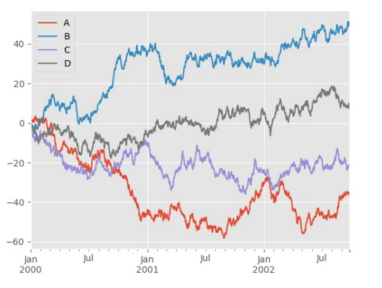
In [135]: ts = pd.Series(np.random.randn(1000), index=pd.date_ra nge('1/1/2000', periods=1000))
In [136]: ts = ts.cumsum()
In [137]: ts.plot()
Out[137]:
<matplotlib.axes._subplots.AxesSubplot at 0x7ff2ab2af5 50>

对于 DataFrame 来说, plot 是一种将所有列及其标签进行绘制的简便方法:
In [138]: df = pd.DataFrame(np.random.randn(1000, 4), index=ts.index,columns=['A', 'B', 'C', 'D'])
In [139]: df = df.cumsum()
In [140]: plt.figure(); df.plot(); plt.legend(loc='best')
Out[140]:
<matplotlib.legend.Legend at 0x7ff29c8163d0>
0.12 导入和保存数据
0.12.1 CSV
参考:写入 CSV 文件。
1、 写入 csv 文件:
In [141]: df.to_csv('foo.csv')
2、 从 csv 文件中读取:
 In [142]: pd.read_csv('foo.csv')
 Out[142]:
 Unnamed: 0 	A 		B 		C 		D
 0 2000-01-01 0.266457 -0.399641 -0.219582 1.186860
 1 2000-01-02 -1.170732 -0.345873 1.653061 -0.282953
 2 2000-01-03 -1.734933 0.530468 2.060811 -0.515536
 3 2000-01-04 -1.555121 1.452620 0.239859 -1.156896
 4 2000-01-05 0.578117 0.511371 0.103552 -2.428202
 5 2000-01-06 0.478344 0.449933 -0.741620 -1.962409
 6 2000-01-07 1.235339 -0.091757 -1.543861 -1.084753
  .. ... ... ... ... ...
  993 2002-09-20 -10.628548 -9.153563 -7.883146 28.313940
  994 2002-09-21 -10.390377 -8.727491 -6.399645 30.914107
  995 2002-09-22 -8.985362 -8.485624 -4.669462 31.367740
  996 2002-09-23 -9.558560 -8.781216 -4.499815 30.518439
  997 2002-09-24 -9.902058 -9.340490 -4.386639 30.105593
  998 2002-09-25 -10.216020 -9.480682 -3.933802 29.758560
  999 2002-09-26 -11.856774 -10.671012 -3.216025 29.369368
  [1000 rows x 5 columns]
0.12.2 HDF5
参考:HDF5 存储
1、 写入 HDF5 存储:
In [143]: df.to_hdf('foo.h5','df')
2、 从 HDF5 存储中读取:
In [144]: pd.read_hdf('foo.h5','df')
Out[144]:
				A 		B 		C 		D
2000-01-01 0.266457 -0.399641 -0.219582 1.186860
2000-01-02 -1.170732 -0.345873 1.653061 -0.282953
2000-01-03 -1.734933 0.530468 2.060811 -0.515536
2000-01-04 -1.555121 1.452620 0.239859 -1.156896
2000-01-05 0.578117 0.511371 0.103552 -2.428202
2000-01-06 0.478344 0.449933 -0.741620 -1.962409
2000-01-07 1.235339 -0.091757 -1.543861 -1.084753
 ... ... ... ... ...
 2002-09-20 -10.628548 -9.153563 -7.883146 28.313940
 2002-09-21 -10.390377 -8.727491 -6.399645 30.914107
 2002-09-22 -8.985362 -8.485624 -4.669462 31.367740
 2002-09-23 -9.558560 -8.781216 -4.499815 30.518439
 2002-09-24 -9.902058 -9.340490 -4.386639 30.105593
 2002-09-25 -10.216020 -9.480682 -3.933802 29.758560
 2002-09-26 -11.856774 -10.671012 -3.216025 29.369368
 [1000 rows x 4 columns]
0.12.3 Excel
参考:MS Excel
1、 写入excel文件:
In [145]: df.to_excel('foo.xlsx', sheet_name='Sheet1')
2、 从excel文件中读取:
In [146]: pd.read_excel('foo.xlsx', 'Sheet1', index_col=None, na_values=['NA'])
Out[146]:
 				A 		B 		C 		D
 2000-01-01 0.266457 -0.399641 -0.219582 1.186860
 2000-01-02 -1.170732 -0.345873 1.653061 -0.282953
 2000-01-03 -1.734933 0.530468 2.060811 -0.515536
 2000-01-04 -1.555121 1.452620 0.239859 -1.156896
 2000-01-05 0.578117 0.511371 0.103552 -2.428202
 2000-01-06 0.478344 0.449933 -0.741620 -1.962409
 2000-01-07 1.235339 -0.091757 -1.543861 -1.084753
 ... ... ... ... ...
 2002-09-20 -10.628548 -9.153563 -7.883146 28.313940
 2002-09-21 -10.390377 -8.727491 -6.399645 30.914107
 2002-09-22 -8.985362 -8.485624 -4.669462 31.367740
 2002-09-23 -9.558560 -8.781216 -4.499815 30.518439
 2002-09-24 -9.902058 -9.340490 -4.386639 30.105593
 2002-09-25 -10.216020 -9.480682 -3.933802 29.758560
 2002-09-26 -11.856774 -10.671012 -3.216025 29.369368
 [1000 rows x 4 columns]
0.14 陷阱
如果你尝试某个操作并且看到如下异常:
 >>> if pd.Series([False, True, False]):
	print("I was true")
Traceback
...
ValueError: The truth value of an array is ambiguous. Use a.empty, a.any() or a.all().
Pandas 秘籍
原文:Pandas cookbook
译者:飞龙 45
第一章 从 CSV 文件中读取数据
原文:Chapter 1
译者:飞龙
协议:CC BY-NC-SA 4.0
import pandas as pd
pd.set_option('display.mpl_style', 'default') # 使图表漂亮一些 figsize(15, 5)
1.1 从 CSV 文件中读取数据
您可以使用 read_csv 函数从CSV文件读取数据。 默认情况下,它假定字段以逗 号分隔。
我们将从蒙特利尔(Montréal)寻找一些骑自行车的数据。 这是原始页面(法 语),但它已经包含在此仓库中。 我们使用的是 2012 年的数据。
这个数据集是一个列表,蒙特利尔的 7 个不同的自行车道上每天有多少人。
broken_df = pd.read_csv('../data/bikes.csv')
In [3]:
# 查看前三行
broken_df[:3]
Date;Berri 1;Br?beuf (donn?es non disponibles);C?te-Sainte-Catherine;Maisonneuve 1;Maisonneuve 2;du Parc;Pierre-Dupuy;Rachel1;St-Urbain (donn?es non disponibles)
0 01/01/2012;35;;0;38;51;26;10;16;
1 02/01/2012;83;;1;68;153;53;6;43;
2 03/01/2012;135;;2;104;248;89;3;58;
你可以看到这完全损坏了。 read_csv 拥有一堆选项能够让我们修复它,在这里我 们:
- 将列分隔符改成 ; sep=’;’
- 将编码改为 latin1 (默认为 utf-8 ) encoding=‘latin1’
- 解析 Date 列中的日期 parse_dates=[‘Date’]
- 告诉它我们的日期将日放在前面,而不是月 dayfirst=True
- 将索引设置为 Date index_col=‘Date’
fixed_df = pd.read_csv('../data/bikes.csv', sep=';', encoding='latin1', parse_dates=['Date'], dayfirst=True, index_col='Date')
fixed_df[:3]
| Berri 1 | Brébeuf (données non disponibles) | C?te- Sainte- Catherine | Maisonneuve 1 | Maisonneuve 2 | |
|---|---|---|---|---|---|
| Date | |||||
| 2012- 01-01 | 35 | NaN | 0 | 38 | 51 |
| 2012- 01-02 | 83 | NaN | 1 | 68 | 153 |
| 2012- 01-03 | 135 | NaN | 2 | 104 | 248 |
1.2 选择一列
当你读取 CSV 时,你会得到一种称为 DataFrame 的对象,它由行和列组成。 您 从数据框架中获取列的方式与从字典中获取元素的方式相同。
这里有一个例子:
fixed_df['Berri 1'] # 提取series
Date
2012-01-01 35
2012-01-02 83
2012-01-03 135
2012-01-04 144
2012-01-05 197
2012-01-06 146
2012-01-07 98
2012-01-08 95
2012-01-09 244
2012-01-10 397
2012-01-11 273
2012-01-12 157
2012-01-13 75
2012-01-14 32
2012-01-15 54
 ...
2012-10-22 3650
2012-10-23 4177
2012-10-24 3744
2012-10-25 3735
2012-10-26 4290
2012-10-27 1857
2012-10-28 1310
2012-10-29 2919
2012-10-30 2887
2012-10-31 2634
2012-11-01 2405
2012-11-02 1582
2012-11-03 844
2012-11-04 966
2012-11-05 2247
Name: Berri 1, Length: 310, dtype: int64
1.3 绘制一列
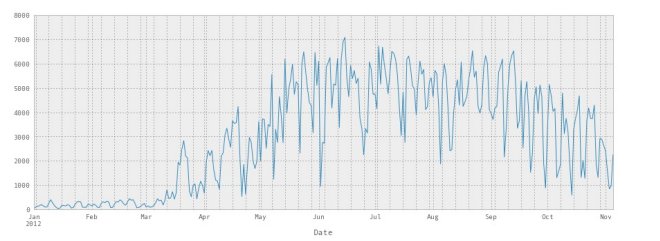
只需要在末尾添加 .plot() ,再容易不过了。
我们可以看到,没有什么意外,一月、二月和三月没有什么人骑自行车。
fixed_df['Berri 1'].plot()
<matplotlib.axes.AxesSubplot at 0x3ea1490>
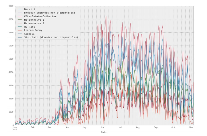
我们也可以很容易地绘制所有的列。 我们会让它更大一点。 你可以看到它挤在一 起,但所有的自行车道基本表现相同 - 如果对骑自行车的人来说是一个糟糕的一 天,任意地方都是糟糕的一天。
fixed_df.plot(figsize=(15, 10))
<matplotlib.axes.AxesSubplot at 0x3fc2110> 49
1.4 将它们放到一起
下面是我们的所有代码,我们编写它来绘制图表:
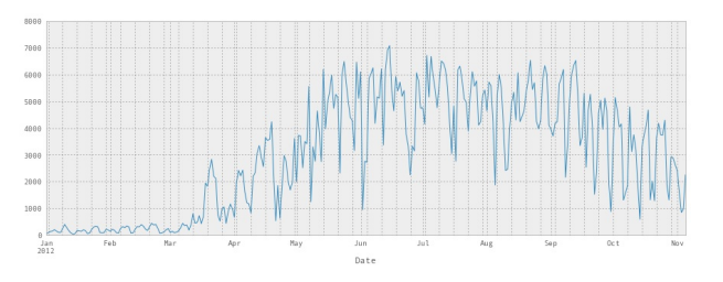
df = pd.read_csv('../data/bikes.csv', sep=';', encoding='latin1' , parse_dates=['Date'], dayfirst=True, index_col='Date')
df['Berri 1'].plot()
<matplotlib.axes.AxesSubplot at 0x4751750> 50
第二章 查看大型数据框架
原文:Chapter 2
译者:飞龙
协议:CC BY-NC-SA 4.0
# 通常的开头
import pandas as pd
# 使图表更大更漂亮
pd.set_option('display.mpl_style', 'default')
pd.set_option('display.line_width', 5000)
pd.set_option('display.max_columns', 60)
figsize(15, 5)
我们将在这里使用一个新的数据集,来演示如何处理更大的数据集。 这是来自 NYC Open Data 的 311 个服务请求的子集。
complaints = pd.read_csv('../data/311-service-requests.csv')
2.1 里面究竟有什么?(总结)
当你查看一个大型数据框架,而不是显示数据框架的内容,它会显示一个摘要。 这 包括所有列,以及每列中有多少非空值。
complaints
<class 'pandas.core.frame.DataFrame'>
Int64Index: 111069 entries, 0 to 111068
Data columns (total 52 columns):
Unique Key 111069 non-null values
Created Date 111069 non-null values
Closed Date 60270 non-null values
Agency 111069 non-null values
Agency Name 111069 non-null values
Complaint Type 111069 non-null values
Descriptor 111068 non-null values
Location Type 79048 non-null values
Incident Zip 98813 non-null values
Incident Address 84441 non-null values
Street Name 84438 non-null values
Cross Street 1 84728 non-null values
Cross Street 2 84005 non-null values
Intersection Street 1 19364 non-null values
Intersection Street 2 19366 non-null values
Address Type 102247 non-null values
City 98860 non-null values
Landmark 95 non-null values
Facility Type 110938 non-null values
Status 111069 non-null values
Due Date 39239 non-null values
Resolution Action Updated Date 96507 non-null values
Community Board 111069 non-null values
Borough 111069 non-null values
X Coordinate (State Plane) 98143 non-null values
Y Coordinate (State Plane) 98143 non-null values
Park Facility Name 111069 non-null values
Park Borough 111069 non-null values
School Name 111069 non-null values
School Number 111052 non-null values
School Region 110524 non-null values
School Code 110524 non-null values
School Phone Number 111069 non-null values
School Address 111069 non-null values
School City 111069 non-null values
School State 111069 non-null values
School Zip 111069 non-null values
School Not Found 38984 non-null values
School or Citywide Complaint 0 non-null values
Vehicle Type 99 non-null values
Taxi Company Borough 117 non-null values
Taxi Pick Up Location 1059 non-null values
Bridge Highway Name 185 non-null values
Bridge Highway Direction 185 non-null values
Road Ramp 184 non-null values
Bridge Highway Segment 223 non-null values
Garage Lot Name 49 non-null values
Ferry Direction 37 non-null values
Ferry Terminal Name 336 non-null values
Latitude 98143 non-null values
Longitude 98143 non-null values
Location 98143 non-null values
dtypes: float64(5), int64(1), object(46)
2.2 选择列和行
为了选择一列,使用列名称作为索引,像这样:
complaints['Complaint Type']
0 Noise - Street/Sidewalk
1 Illegal Parking
2 Noise - Commercial
3 Noise - Vehicle
4 Rodent
5 Noise - Commercial
6 Blocked Driveway
7 Noise - Commercial
8 Noise - Commercial
9 Noise - Commercial
10 Noise - House of Worship
11 Noise - Commercial
12 Illegal Parking
13 Noise - Vehicle
14 Rodent
...
111054 Noise - Street/Sidewalk
111055 Noise - Commercial
111056 Street Sign - Missing
111057 Noise
111058 Noise - Commercial
111059 Noise - Street/Sidewalk
111060 Noise
111061 Noise - Commercial
111062 Water System
111063 Water System
111064 Maintenance or Facility
111065 Illegal Parking
111066 Noise - Street/Sidewalk
111067 Noise - Commercial
111068 Blocked Driveway
Name: Complaint Type, Length: 111069, dtype: object
要获得 DataFrame 的前 5 行,我们可以使用切片: df [:5] 。
这是一个了解数据框架中存在什么信息的很好方式 - 花一点时间来查看内容并获得 此数据集的感觉。
complaints[:5]
| Unique Key | Created Date | Closed Date | Agency | Agency Name | Complaint Type | |
|---|---|---|---|---|---|---|
| 0 | 26589651 | 10/31/2013 02:08:41 AM | NaN | NYPD | New York City Police Department | Noise - Street/Sidewalk |
| 1 | 26593698 | 10/31/2013 02:01:04 AM | NaN | NYPD | New York City Police Department | Illegal Parking |
| 2 | 26594139 | 10/31/2013 02:00:24 AM | 10/31/2013 02:40:32 AM | NYPD | New York City Police Department | Noise - Commercial |
| 3 | 26595721 | 10/31/2013 01:56:23 AM | 10/31/2013 02:21:48 AM | NYPD | New York City Police Department | Noise - Vehicle |
| 4 | 26590930 | 10/31/2013 01:53:44 AM | NaN | DOHMH | Department of Health and Mental Hygiene | Rodent |
我们可以组合它们来获得一列的前五行。
 complaints['Complaint Type'][:5]
 0 Noise - Street/Sidewalk
 1 Illegal Parking
 2 Noise - Commercial
 3 Noise - Vehicle
 4 Rodent
 Name: Complaint Type, dtype: object
并且无论我们以什么方向:
 complaints[:5]['Complaint Type']
0 Noise - Street/Sidewalk
1 Illegal Parking
2 Noise - Commercial
3 Noise - Vehicle
4 Rodent
Name: Complaint Type, dtype: object
2.3 选择多列
如果我们只关心投诉类型和区,但不关心其余的信息怎么办? Pandas 使它很容易选择列的一个子集:只需将所需列的列表用作索引。
complaints[['Complaint Type', 'Borough']]
<class 'pandas.core.frame.DataFrame'>
Int64Index: 111069 entries, 0 to 111068
Data columns (total 2 columns):
Complaint Type 111069 non-null values
Borough 111069 non-null values
dtypes: object(2)
这会向我们展示总结,我们可以获取前 10 列:
complaints[['Complaint Type', 'Borough']][:10]
	Complaint Type 			Borough
0 Noise - Street/Sidewalk 	QUEENS
1 Illegal Parking 			QUEENS
2 Noise - Commercial 		MANHATTAN
3 Noise - Vehicle 			MANHATTAN
4 Rodent 					MANHATTAN
5 Noise - Commercial 		QUEENS
6 Blocked Driveway 			QUEENS
7 Noise - Commercial 		QUEENS
8 Noise - Commercial 		MANHATTAN
9 Noise - Commercial 		BROOKLYN
2.4 什么是最常见的投诉类型?
这是个易于回答的问题,我们可以调用 .value_counts() 方法:
complaints['Complaint Type'].value_counts()
HEATING 						14200
GENERAL CONSTRUCTION 			7471
Street Light Condition 			7117
DOF Literature Request 			5797
PLUMBING 						5373
PAINT - PLASTER 				5149
Blocked Driveway 				4590
NONCONST 						3998
Street Condition 				3473
Illegal Parking 				3343
Noise 							3321
Traffic Signal Condition 		3145
Dirty Conditions 				2653
Water System 					2636
Noise - Commercial 				2578
...
Opinion for the Mayor 			2
Window Guard 					2
DFTA Literature Request 		2
Legal Services Provider Complaint 2
Open Flame Permit 				1
Snow 1 Municipal Parking Facility 1
X-Ray Machine/Equipment 		1
Stalled Sites 					1
DHS Income Savings Requirement 1
Tunnel Condition 				1
Highway Sign - Damaged 			1
Ferry Permit 					1
Trans Fat 						1
DWD 							1
Length: 165, dtype: int64
如果我们想要最常见的 10 个投诉类型,我们可以这样:
 complaint_counts = complaints['Complaint Type'].value_counts()
 complaint_counts[:10]
HEATING 14200
GENERAL CONSTRUCTION 7471
Street Light Condition 7117
DOF Literature Request 5797
PLUMBING 5373
PAINT - PLASTER 5149
Blocked Driveway 4590
NONCONST 3998
Street Condition 3473
Illegal Parking 3343
dtype: int64
但是还可以更好,我们可以绘制出来!
 complaint_counts[:10].plot(kind='bar')
  <matplotlib.axes.AxesSubplot at 0x7ba2290> 60

第三章 继续探索噪音投诉
原文:Chapter 3
译者:飞龙
协议:CC BY-NC-SA 4.0
# 通常的开头
import pandas as pd
# 使图表更大更漂亮
pd.set_option('display.mpl_style', 'default') figsize(15, 5)
# 始终展示所有列
pd.set_option('display.line_width', 5000)
pd.set_option('display.max_columns', 60)
让我们继续 NYC 311 服务请求的例子。
complaints = pd.read_csv('../data/311-service-requests.csv')
3.1 仅仅选择噪音投诉
我想知道哪个区有最多的噪音投诉。 首先,我们来看看数据,看看它是什么样子:
complaints[:5]
Unique Key Created Date Closed Date Agency Agency Name Complaint Type
0 26589651 10/31/2013 02:08:41 AM NaN NYPD New York City Police Department Noise - Street/Sidewalk
1 26593698 10/31/2013 02:01:04 AM NaN NYPD New York City Police Department Illegal Parking
2 26594139 10/31/2013 02:00:24 AM 10/31/2013 02:40:32 AM NYPD New York City Police Department Noise - Commercial
3 26595721 10/31/2013 01:56:23 AM 10/31/2013 02:21:48 AM NYPD New York City Police Department Noise - Vehicle
4 26590930 10/31/2013 01:53:44 AM NaN DOHMH Department of Health and Mental Hygiene Rodent
为了得到噪音投诉,我们需要找到 Complaint Type 列为 Noise - Street/Sidewalk 的行。 我会告诉你如何做,然后解释发生了什么。
noise_complaints = complaints[complaints['Complaint Type'] == "N oise - Street/Sidewalk"] noise_complaints[:3]
Unique Key Created Date Closed Date Agency Agency Name Complaint
0 26589651 10/31/2013 02:08:41 AM NaN NYPD New York City Police Department Noise - Street/Sidewalk
16 26594086 10/31/2013 12:54:03 AM 10/31/2013 02:16:39 AM NYPD New York City Police Department Noise - Street/Sidewalk
25 26591573 10/31/2013 12:35:18 AM 10/31/2013 02:41:35 AM NYPD New York City Police Department Noise - Street/Sidewalk
如果你查看 noise_complaints ,你会看到它生效了,它只包含带有正确的投诉 类型的投诉。 但是这是如何工作的? 让我们把它解构成两部分
complaints['Complaint Type'] == "Noise - Street/Sidewalk"
0 True
1 False
2 False
3 False
4 False
5 False
6 False
7 False
8 False
9 False
10 False
11 False
12 False
13 False
14 False
 ...
111054 True
111055 False
111056 False
111057 False
111058 False
111059 True
111060 False
111061 False
111062 False
111063 False
111064 False
111065 False
111066 True
111067 False
111068 False
Name: Complaint Type, Length: 111069, dtype: bool
这是一个 True 和 False 的大数组,对应 DataFrame 中的每一行。 当我们用这 个数组索引我们的 DataFrame 时,我们只得到其中为 True 行。 您还可以将多个条件与 & 运算符组合,如下所示:
is_noise = complaints['Complaint Type'] == "Noise - Street/Sidew alk"
in_brooklyn = complaints['Borough'] == "BROOKLYN"
complaints[is_noise & in_brooklyn][:5]
Unique Key Created Date Closed Date Agency Agency Name Complaint
31 26595564 10/31/2013 12:30:36 AM NaN NYPD New York City Police Department Noise - Street/Sidewalk
49 26595553 10/31/2013 12:05:10 AM 10/31/2013 02:43:43 AM NYPD New York City Police Department Noise - Street/Sidewalk
109 26594653 10/30/2013 11:26:32 PM 10/31/2013 12:18:54 AM NYPD New York City Police Department Noise - Street/Sidewalk
236 26591992 10/30/2013 10:02:58 PM 10/30/2013 10:23:20 PM NYPD New York City Police Department Noise - Street/Sidewalk
370 26594167 10/30/2013 08:38:25 PM 10/30/2013 10:26:28 PM NYPD New York City Police Department Noise - Street/Sidewalk
或者如果我们只需要几列:
complaints[is_noise & in_brooklyn][['Complaint Type', 'Borough', 'Created Date', 'Descriptor']][:10]
	Complaint Type 			Borough 	Created Date 		Descriptor
31 Noise - Street/Sidewalk BROOKLYN 10/31/2013 12:30:36 AM Loud Music/Party
49 Noise - Street/Sidewalk BROOKLYN 10/31/2013 12:05:10 AM Loud Talking
109 Noise - Street/Sidewalk BROOKLYN 10/30/2013 11:26:32 PM Loud Music/Party
236 Noise - Street/Sidewalk BROOKLYN 10/30/2013 10:02:58 PM Loud Talking
370 Noise - Street/Sidewalk BROOKLYN 10/30/2013 08:38:25 PM Loud Music/Party
378 Noise - Street/Sidewalk BROOKLYN 10/30/2013 08:32:13 PM Loud Talking
656 Noise - Street/Sidewalk BROOKLYN 10/30/2013 06:07:39 PM Loud Music/Party
1251 Noise - Street/Sidewalk BROOKLYN 10/30/2013 03:04:51 PM Loud Talking
5416 Noise - Street/Sidewalk BROOKLYN 10/29/2013 10:07:02 PM Loud Talking
5584 Noise - Street/Sidewalk BROOKLYN 10/29/2013 08:15:59 PM Loud Music/Party
3.2 numpy 数组的注解
在内部,列的类型是 pd.Series 。
pd.Series([1,2,3])
 0 1
 1 2
 2 3
 dtype: int64
而且 pandas.Series 的内部是 numpy 数组。 如果将 .values 添加到任何 Series 的末尾,你将得到它的内部 numpy 数组。
np.array([1,2,3])
array([1, 2, 3])
pd.Series([1,2,3]).values
array([1, 2, 3])
所以这个二进制数组选择的操作,实际上适用于任何 NumPy 数组:
arr = np.array([1,2,3])
arr != 2
array([ True, False, True], dtype=bool)
arr[arr != 2]
array([1, 3])
3.3 所以,哪个区的噪音投诉最多?
is_noise = complaints['Complaint Type'] == "Noise - Street/Sidew alk"
noise_complaints = complaints[is_noise] noise_complaints['Borough'].value_counts()
MANHATTAN 917
BROOKLYN 456
BRONX 292
QUEENS 226
STATEN ISLAND 36
Unspecified 1
dtype: int64
这是曼哈顿! 但是,如果我们想要除以总投诉数量,以使它有点更有意义? 这也 很容易:
noise_complaint_counts = noise_complaints['Borough'].value_count s()
complaint_counts = complaints['Borough'].value_counts()
noise_complaint_counts / complaint_counts
BRONX 0
BROOKLYN 0
MANHATTAN 0
QUEENS 0
STATEN ISLAND 0
Unspecified 0
dtype: int64
糟糕,为什么是零?这是因为 Python 2 中的整数除法。让我们通过 将 complaints_counts 转换为浮点数组来解决它。
noise_complaint_counts / complaint_counts.astype(float)
BRONX 0.014833
BROOKLYN 0.013864
MANHATTAN 0.037755
QUEENS 0.010143
STATEN ISLAND 0.007474
Unspecified 0.000141
dtype: float64
(noise_complaint_counts / complaint_counts.astype(float)).plot(k ind='bar')
<matplotlib.axes.AxesSubplot at 0x75b7890>

所以曼哈顿的噪音投诉比其他区要多。
第四章 蒙特利尔的骑手
原文:Chapter 4
译者:飞龙
协议:CC BY-NC-SA 4.0
 import pandas as pd
 pd.set_option('display.mpl_style', 'default')
 # 使图表漂亮一些
 figsize(15, 5)
好的! 我们将在这里回顾我们的自行车道数据集。 我住在蒙特利尔,我很好奇我 们是一个通勤城市,还是以骑自行车为乐趣的城市 - 人们在周末还是工作日骑自行 车?
4.1 向我们的 DataFrame 中刚添加 weekday 列
首先我们需要加载数据,我们之前已经做过了。
 bikes = pd.read_csv('../data/bikes.csv', sep=';', encoding='lati n1', parse_dates=['Date'], dayfirst=True, index_col='Date')
 bikes['Berri 1'].plot()
 <matplotlib.axes.AxesSubplot at 0x30d8610>

接下来,我们只是看看 Berri 自行车道。 Berri 是蒙特利尔的一条街道,是一个相当 重要的自行车道。 现在我习惯走这条路去图书馆,但我在旧蒙特利尔工作时,我习惯于走这条路去上班。
所以我们要创建一个只有 Berri 自行车道的 DataFrame 。
berri_bikes = bikes[['Berri 1']]
berri_bikes[:5]
			Berri 1
Date
2012-01-01 35
2012-01-02 83
2012-01-03 135
2012-01-04 144
2012-01-05 197
接下来,我们需要添加一列 weekday 。 首先,我们可以从索引得到星期。 我们还没有谈到索引,但索引在上面的 DataFrame 中是左边的东西,在 Date 下面。 它 基本上是一年中的所有日子。
berri_bikes.index
<class 'pandas.tseries.index.DatetimeIndex'>
[2012-01-01 00:00:00, ..., 2012-11-05 00:00:00]
Length: 310, Freq: None, Timezone: None
你可以看到,实际上缺少一些日期 - 实际上只有一年的 310 天。 天知道为什么。 Pandas 有一堆非常棒的时间序列功能,所以如果我们想得到每一行的月份中的日 期,我们可以这样做:
berri_bikes.index.day
array([ 1, 2, 3, 4, 5, 6, 7, 8, 9, 10, 11, 12, 13, 14, 1 5, 16, 17, 18, 19, 20, 21, 22, 23, 24, 25, 26, 27, 28, 29, 30, 31, 1, 2, 3,4, 5, 6, 7, 8, 9, 10, 11, 12, 13, 14, 15, 16, 17, 1 8, 19, 20, 21, 22, 23, 24, 25, 26, 27, 28, 29, 1, 2, 3, 4, 5, 6, 7, 8,9, 10, 11, 12, 13, 14, 15, 16, 17, 18, 19, 20, 21, 22, 2 3, 24, 25, 26, 27, 28, 29, 30, 31, 1, 2, 3, 4, 5, 6, 7, 8, 9, 10, 11, 12, 13, 14, 15, 16, 17, 18, 19, 20, 21, 22, 23, 24, 25, 2 6, 27, 28, 29, 30, 1, 2, 3, 4, 5, 6, 7, 8, 9, 10, 11, 12, 1 3, 14, 15, 16, 17, 18, 19, 20, 21, 22, 23, 24, 25, 26, 27, 28, 29, 3 0, 31, 1,2, 3, 4, 5, 6, 7, 8, 9, 10, 11, 12, 13, 14, 15, 1 6, 17, 18, 19, 20, 21, 22, 23, 24, 25, 26, 27, 28, 29, 30, 1, 2, 3, 4, 5,6, 7, 8, 9, 10, 11, 12, 13, 14, 15, 16, 17, 18, 19, 2 0, 21, 22, 23, 24, 25, 26, 27, 28, 29, 30, 31, 1, 2, 3, 4, 5, 6, 7, 8,9, 10, 11, 12, 13, 14, 15, 16, 17, 18, 19, 20, 21, 22, 2 3, 24, 25, 26, 27, 28, 29, 30, 31, 1, 2, 3, 4, 5, 6, 7, 8, 9, 10, 11, 12, 13, 14, 15, 16, 17, 18, 19, 20, 21, 22, 23, 24, 25, 2 6, 27, 28, 29, 30, 1, 2, 3, 4, 5, 6, 7, 8, 9, 10, 11, 12, 1 3, 14, 15, 16, 17, 18, 19, 20, 21, 22, 23, 24, 25, 26, 27, 28, 29, 3 0, 31, 1,2, 3, 4, 5], dtype=int32)
我们实际上想要星期:
berri_bikes.index.weekday
array([6, 0, 1, 2, 3, 4, 5, 6, 0, 1, 2, 3, 4, 5, 6, 0, 1, 2, 3, 4 , 5, 6, 0, 1, 2, 3, 4, 5, 6, 0, 1, 2, 3, 4, 5, 6, 0, 1, 2, 3, 4, 5, 6 , 0, 1, 2, 3, 4, 5, 6, 0, 1, 2, 3, 4, 5, 6, 0, 1, 2, 3, 4, 5, 6, 0, 1 , 2, 3, 4, 5, 6, 0, 1, 2, 3, 4, 5, 6, 0, 1, 2, 3, 4, 5, 6, 0, 1, 2, 3 , 4, 5, 6, 0, 1, 2, 3, 4, 5, 6, 0, 1, 2, 3, 4, 5, 6, 0, 1, 2, 3, 4, 5 , 6, 0, 1, 2, 3, 4, 5, 6, 0, 1, 2, 3, 4, 5, 6, 0, 1, 2, 3, 4, 5, 6, 0 , 1, 2, 3, 4, 5, 6, 0, 1, 2, 3, 4, 5, 6, 0, 1, 2, 3, 4, 5, 6, 0, 1, 2 , 3, 4, 5, 6, 0, 1, 2, 3, 4, 5, 6, 0, 1, 2, 3, 4, 5, 6, 0, 1, 2, 3, 4 , 5, 6, 0, 1, 2, 3, 4, 5, 6, 0, 1, 2, 3, 4, 5, 6, 0, 1, 2, 3, 4, 5, 6 , 0, 1, 2, 3, 4, 5, 6, 0, 1, 2, 3, 4, 5, 6, 0, 1, 2, 3, 4, 5, 6, 0, 1 , 2, 3, 4, 5, 6, 0, 1, 2, 3, 4, 5, 6, 0, 1, 2, 3, 4, 5, 6, 0, 1, 2, 3 , 4, 5, 6, 0, 1, 2, 3, 4, 5, 6, 0, 1, 2, 3, 4, 5, 6, 0, 1, 2, 3, 4, 5 , 6, 0, 1, 2, 3, 4, 5, 6, 0, 1, 2, 3, 4, 5, 6, 0, 1, 2, 3, 4, 5, 6, 0 , 1, 2, 3, 4, 5, 6, 0, 1, 2, 3, 4, 5, 6, 0], dtype=int32)
这是周中的日期,其中 0 是星期一。我通过查询日历得到 0 是星期一。 现在我们知道了如何获取星期,我们可以将其添加到我们的 DataFrame 中作为一 列:
berri_bikes['weekday'] = berri_bikes.index.weekday
berri_bikes[:5]
				Berri 1 	weekday
Date
2012-01-01 		35 			6
2012-01-02 		83 			0
2012-01-03 		135 		1
2012-01-04 		144 		2
2012-01-05 		197 		3
4.2 按星期统计骑手
这很易于实现! Dataframe 有一个类似于 SQL groupby 的 .groupby() 方法,如果你熟悉的 话。 我现在不打算解释更多 - 如果你想知道更多,请见文档。
在这种情况下, berri_bikes.groupby(‘weekday’) .aggregate(sum)`意味着“按 星期对行分组,然后将星期相同的所有值相加”。
weekday_counts = berri_bikes.groupby('weekday').aggregate(sum)
weekday_counts
Berri 1 weekday
0 134298
1 135305
2 152972
3 160131
4 141771
5 101578
6 99310
很难记住 0, 1, 2, 3, 4, 5, 6 是什么,所以让我们修复它并绘制出来:
weekday_counts.index = ['Monday', 'Tuesday', 'Wednesday', 'Thurs day', 'Friday', 'Saturday', 'Sunday']
weekday_counts
Berri 1
Monday 134298
Tuesday 135305
Wednesday 152972
Thursday 160131
Friday 141771
Saturday 101578
Sunday 99310
weekday_counts.plot(kind='bar')
<matplotlib.axes.AxesSubplot at 0x3216a90>

所以看起来蒙特利尔是通勤骑自行车的人 - 他们在工作日骑自行车更多。
4.3 放到一起
让我们把所有的一起,证明它是多么容易。 6 行的神奇 Pandas!
如果你想玩一玩,尝试将 sum 变为 max , np.median ,或任何你喜欢的其他函 数。
bikes = pd.read_csv('../data/bikes.csv', sep=';', encoding='latin1', parse_dates=['Date'], dayfirst=True, index_col='Date')
# 添加 weekday 列
berri_bikes = bikes[['Berri 1']]
berri_bikes['weekday'] = berri_bikes.index.weekday
# 按照星期累计骑手,并绘制出来
weekday_counts = berri_bikes.groupby('weekday').aggregate(sum)
weekday_counts.index = ['Monday', 'Tuesday', 'Wednesday', 'Thurs day', 'Friday', 'Saturday', 'Sunday'] weekday_counts.plot(kind='bar')
第五章 蒙特利尔的天气 - 日期操作
原文:Chapter 5
译者:飞龙
协议:CC BY-NC-SA 4.0
5.1 下载一个月的天气数据
在处理自行车数据时,我需要温度和降水数据,来弄清楚人们下雨时是否喜欢骑自行车。 所以我访问了加拿大历史天气数据的网站,并想出如何自动获得它们。
这里我们将获取 2012年 3 月的数据,并清理它们。
以下是可用于在蒙特利尔获取数据的网址模板。
url_template = "http://climate.weather.gc.ca/climateData/bulkdat a_e.html?format=csv&stationID=5415&Year={year}&Month={month}&tim eframe=1&submit=Download+Data"
我们获取 2012年三月的数据,我们需要以 month=3, year=2012 对它格式化:
url = url_template.format(month=3, year=2012) weather_mar2012 = pd.read_csv(url, skiprows=16, index_col='Date/Time', parse_dates=True, encoding='latin1')
这非常不错! 我们可以使用和以前一样的 read_csv 函数,并且只是给它一个 URL 作为文件名。 真棒。
在这个 CSV 的顶部有 16 行元数据,但是 Pandas 知道 CSV 很奇怪,所以有一 个 skiprows 选项。 我们再次解析日期,并将 Date/Time 设置为索引列。 这是 产生的 DataFrame 。
weather_mar2012
<class 'pandas.core.frame.DataFrame'>
DatetimeIndex: 744 entries, 2012-03-01 00:00:00 to 2012-03-31 23 :00:00
Data columns (total 24 columns):
Year 744 non-null values
Month 744 non-null values
Day 744 non-null values
Time 744 non-null values
Data Quality 744 non-null values
Temp (°C) 744 non-null values
Temp Flag 0 non-null values
Dew Point Temp (°C) 744 non-null values
Dew Point Temp Flag 0 non-null values
Rel Hum (%) 744 non-null values
Rel Hum Flag 0 non-null values
Wind Dir (10s deg) 715 non-null values
Wind Dir Flag 0 non-null values
Wind Spd (km/h) 744 non-null values
Wind Spd Flag 3 non-null values
Visibility (km) 744 non-null values
Visibility Flag 0 non-null values
Stn Press (kPa) 744 non-null values
Stn Press Flag 0 non-null values
Hmdx 12 non-null values
Hmdx Flag 0 non-null values
Wind Chill 242 non-null values
Wind Chill Flag 1 non-null values
Weather 744 non-null values
dtypes: float64(14), int64(5), object(5)
让我们绘制它吧!
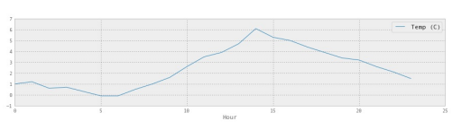
weather_mar2012[u"Temp (\xb0C)"].plot(figsize=(15, 5))
<matplotlib.axes.AxesSubplot at 0x34e8990>

注意它在中间升高到25°C。这是一个大问题。 这是三月,人们在外面穿着短裤。 我出城了,而且错过了。真是伤心啊。
我需要将度数字符 ° 写为 ‘\xb0’ 。 让我们去掉它,让它更容易键入。
weather_mar2012.columns = [s.replace(u'\xb0', '') for s in weath er_mar2012.columns]
你会注意到在上面的摘要中,有几个列完全是空的,或其中只有几个值。 让我们使 用 dropna 去掉它们。
dropna 中的 axis=1 意味着“删除列,而不是行”,以及 how =‘any’ 意味着“如 果任何值为空,则删除列”。
现在更好了 - 我们只有带有真实数据的列。
					Year Month Day Time 	Data Quality Temp (C) Dew Point Temp (C) Rel Hum(%)
Date/Time
2012-03- 0100:00:00 2012 	3 	1 	00:00 		-5.5 				-9.7 				72
2012-03- 0101:00:00 2012 	3 	1 	01:00 		-5.7 				-8.7 				79
2012-03- 0102:00:00 2012 	3 	1 	02:00 		-5.4 				-8.3 				80
2012-03- 0103:00:00 2012 	3 	1 	03:00 		-4.7 				-7.7 				79
2012-03- 0104:00:00 2012 	3 	1 	04:00 		-5.4 				-7.8 				83
Year/Month/Day/Time 列是冗余的,但 Data Quality 列看起来不太有用。 让 我们去掉他们。
axis = 1 参数意味着“删除列”,像以前一样。 dropna 和 drop 等操作的默认值总是对行进行操作。
weather_mar2012 = weather_mar2012.drop(['Year', 'Month', 'Day', 'Time', 'Data Quality'], axis=1)
weather_mar2012[:5]
					Temp (C) Dew Point Temp (C) Rel Hum(%) Wind Spd (km/h) Visibility (km) Stn Press (kPa) Weather
Date/Time
2012-03- 0100:00:00 -5.5 		-9.7 				72 			24 				4.0 			100.97 		Snow
2012-03- 0101:00:00 -5.7 		-8.7 				79 			26 				2.4 			100.87 		Snow
2012-03- 0102:00:00 -5.4 		-8.3 				80 			28 				4.8 			100.80 		Snow
2012-03- 0103:00:00 -4.7 		-7.7 				79 			28 				4.0 			100.69 		Snow
2012-03- 0104:00:00 -5.4 		-7.8 				83 			35 				1.6 			100.62 		Snow
5.2 按一天中的小时绘制温度
这只是为了好玩 - 我们以前已经做过,使用 groupby 和 aggregate ! 我们将了 解它是否在夜间变冷。 好吧,这是显然的。 但是让我们这样做。
temperatures = weather_mar2012[[u'Temp (C)']]
temperatures['Hour'] = weather_mar2012.index.hour
temperatures.groupby('Hour').aggregate(np.median).plot()
所以温度中位数在 2pm 时达到峰值。
5.3 获取整年的数据
好吧,那么如果我们想要全年的数据呢? 理想情况下 API 会让我们下载,但我不 能找出一种方法来实现它。
首先,让我们将上面的成果放到一个函数中,函数按照给定月份获取天气。
我注意到有一个烦人的 bug,当我请求一月时,它给我上一年的数据,所以我们要 解决这个问题。 【真的是这样。你可以检查一下 =)】
def download_weather_month(year, month):
	if month == 1:
		year += 1
	url = url_template.format(year=year, month=month) weather_data = pd.read_csv(url, skiprows=16, index_col='Date /Time', parse_dates=True)
	weather_data = weather_data.dropna(axis=1)
	weather_data.columns = [col.replace('\xb0', '') for col in w eather_data.columns]
	weather_data = weather_data.drop(['Year', 'Day', 'Month', 'T ime', 'Data Quality'], axis=1)
	return weather_data
我们可以测试这个函数是否行为正确:
download_weather_month(2012, 1)[:5]
| Temp © | Dew Point Temp © | Rel Hum(%) | Wind Spd (km/h) | Visibility (km) | Stn Press (kPa) | Weather | |
|---|---|---|---|---|---|---|---|
| Date/Time | |||||||
| 2012-01- 0100:00:00 | -1.8 | -3.9 | 86 | 4 | 8.0 | 101.24 | Fog |
| 2012-01- 0101:00:00 | -1.8 | -3.7 | 87 | 4 | 8.0 | 101.24 | Fog |
| 2012-01- 0102:00:00 | -1.8 | -3.4 | 89 | 7 | 4.0 | 101.26 | Freezing Drizzle,Fog |
| 2012-01- 0103:00:00 | -1.5 | -3.2 | 88 | 6 | 4.0 | 101.27 | Freezing Drizzle,Fog |
| 2012-01- 0104:00:00 | 1.5 | -3.3 | 88 | 7 | 4.8 | 101.23 | Fog |
现在我们一次性获取了所有月份,需要一些时间来运行。
data_by_month = [download_weather_month(2012, i) for i in range(1 , 13)]
一旦我们完成之后,可以轻易使用 pd.concat 将所有 DataFrame 连接成一个 大 DataFrame 。 现在我们有整年的数据了!
weather_2012 = pd.concat(data_by_month)
 weather_2012
<class 'pandas.core.frame.DataFrame'> DatetimeIndex: 8784 entries, 2012-01-01 00:00:00 to 2012-12-31 2 3:00:00
Data columns (total 7 columns):
Temp (C) 8784 non-null values
Dew Point Temp (C) 8784 non-null values
Rel Hum (%) 8784 non-null values
Wind Spd (km/h) 8784 non-null values
Visibility (km) 8784 non-null values
Stn Press (kPa) 8784 non-null values
Weather 8784 non-null values
dtypes: float64(4), int64(2), object(1)
5.4 保存到 CSV
每次下载数据会非常慢,所以让我们保存 DataFrame :
weather_2012.to_csv('../data/weather_2012.csv')
这就完成了!
5.5 总结
在这一章末尾,我们下载了加拿大 2012 年的所有天气数据,并保存到了 CSV 中。
我们通过一次下载一个月份,之后组合所有月份来实现。
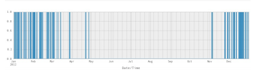
这里是 2012 年每一个小时的天气数据!
 weather_2012_final = pd.read_csv('../data/weather_2012.csv', ind ex_col='Date/Time')
 weather_2012_final['Temp (C)'].plot(figsize=(15, 6))
 <matplotlib.axes.AxesSubplot at 0x345b5d0>

第六章 温度与降雪 - 字符串操作
原文:Chapter 6
译者:飞龙
协议:CC BY-NC-SA 4.0
 import pandas as pd
 pd.set_option('display.mpl_style', 'default')
 figsize(15, 3)
我们前面看到,Pandas 真的很善于处理日期。 它也善于处理字符串! 我们从第 5 章回顾我们的天气数据。
 weather_2012 = pd.read_csv('../data/weather_2012.csv', parse_dat es=True, index_col='Date/Time')
 weather_2012[:5]
| Temp © | Dew Point Temp © | Rel Hum(%) | Wind Spd (km/h) | Visibility (km) | Stn Press (kPa) | Weather | |
|---|---|---|---|---|---|---|---|
| Date/Time | |||||||
| 2012-01- 0100:00:00 | -1.8 | -3.9 | 86 | 4 | 8.0 | 101.24 | Fog |
| 2012-01- 0101:00:00 | -1.8 | -3.7 | 87 | 4 | 8.0 | 101.24 | Fog |
| 2012-01- 0102:00:00 | -1.8 | -3.4 | 89 | 7 | 4.0 | 101.26 | Freezing Drizzle,Fog |
| 2012-01- 0103:00:00 | -1.5 | -3.2 | 88 | 6 | 4.0 | 101.27 | Freezing Drizzle,Fog |
| 2012-01- 0104:00:00 | 1.5 | -3.3 | 88 | 7 | 4.8 | 101.23 | Fog |
6.1 字符串操作
您会看到 Weather 列会显示每小时发生的天气的文字说明。 如果文本描述包 含 Snow ,我们将假设它是下雪的。
pandas 提供了向量化的字符串函数,以便于对包含文本的列进行操作。 文档中有 一些很好的例子。
weather_description = weather_2012['Weather']
is_snowing = weather_description.str.contains('Snow')
这会给我们一个二进制向量,很难看出里面的东西,所以我们绘制它:
# Not super useful is_snowing[:5]
Date/Time
2012-01-01 00:00:00 False
2012-01-01 01:00:00 False
2012-01-01 02:00:00 False
2012-01-01 03:00:00 False
2012-01-01 04:00:00 False
Name: Weather, dtype: bool
# More useful!
is_snowing.plot()
<matplotlib.axes.AxesSubplot at 0x403c190>
6.2 使用 resample
DataFrame.resample(freq, how=None, axis=0, fill_method=None, closed=None, label=None, convention='start',kind=None, loffset=None, limit=None, base=0)
| 参数 | 说明 |
|---|---|
| freq | 表示重采样频率,例如‘M’、‘5min’,Second(15),‘3T’-三分钟 |
| how=‘mean’ | 用于产生聚合值的函数名或数组函数,例如‘mean’、‘ohlc’、np.max等,默认是‘mean’,其他常用的值由:‘first’、‘last’、‘median’、‘max’、‘min’ |
| axis=0 | 默认是纵轴,横轴设置axis=1 |
| fill_method = None | 升采样时如何插值,比如‘ffill’、‘bfill’等 |
| closed = ‘right’ | 在降采样时,各时间段的哪一段是闭合的,‘right’或‘left’,默认‘right’ |
| label= ‘right’ | 在降采样时,如何设置聚合值的标签,例如,9:30-9:35会被标记成9:30还是9:35,默认9:35 |
| loffset = None | 面元标签的时间校正值,比如‘-1s’或Second(-1)用于将聚合标签调早1秒 |
| limit=None | 在向前或向后填充时,允许填充的最大时期数 |
| kind = None | 聚合到时期(‘period’)或时间戳(‘timestamp’),默认聚合到时间序列的索引类型 |
| convention = None | 当重采样时期时,将低频率转换到高频率所采用的约定(start或end)。默认‘end’ |
找到下雪最多的月份 如果我们想要每个月的温度中值,我们可以使用 resample() 方法,如下所示:
weather_2012['Temp (C)'].resample('M', how=np.median).plot(kind= 'bar')
<matplotlib.axes.AxesSubplot at 0x560cc50>

毫无奇怪,七月和八月是最暖和的。
所以我们可以将 is_snowing 转化为一堆 0 和 1,而不是 True 和 False 。
is_snowing.astype(float)
Date/Time
2012-01-01 00:00:00 0
2012-01-01 01:00:00 0
2012-01-01 02:00:00 0
2012-01-01 03:00:00 0
2012-01-01 04:00:00 0
2012-01-01 05:00:00 0
2012-01-01 06:00:00 0
2012-01-01 07:00:00 0
2012-01-01 08:00:00 0
2012-01-01 09:00:00 0
Name: Weather, dtype: float64
然后使用 resample 寻找每个月下雪的时间比例。
is_snowing.astype(float).resample('M', how=np.mean)
Date/Time
2012-01-31 0.240591
2012-02-29 0.162356
2012-03-31 0.087366
2012-04-30 0.015278
2012-05-31 0.000000
2012-06-30 0.000000
2012-07-31 0.000000
2012-08-31 0.000000
2012-09-30 0.000000
2012-10-31 0.000000
2012-11-30 0.038889
2012-12-31 0.251344
Freq: M, dtype: float64
is_snowing.astype(float).resample('M', how=np.mean).plot(kind='b ar')
<matplotlib.axes.AxesSubplot at 0x5bdedd0>
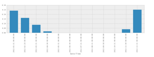
所以现在我们知道了! 2012 年 12 月是下雪最多的一个月。 此外,这个图表暗示 着我感觉到的东西 - 11 月突然开始下雪,然后慢慢变慢,需要很长时间停止,最后 下雪的月份通常在 4 月或 5 月。
6.3 将温度和降雪绘制在一起
我们还可以将这两个统计(温度和降雪)合并为一个 DataFrame ,并将它们绘制 在一起:
temperature = weather_2012['Temp (C)'].resample('M', how=np.median)
is_snowing = weather_2012['Weather'].str.contains('Snow')
snowiness = is_snowing.astype(float).resample('M', how=np.mean)
# Name the columns
temperature.name = "Temperature"
snowiness.name = "Snowiness"
我们再次使用 concat ,将两个统计连接为一个 DataFrame 。
stats = pd.concat([temperature, snowiness], axis=1)
stats
			Temperature 	Snowiness
Date/Time
2012-01-31 -7.05 			0.240591
2012-02-29 -4.10 			0.162356
2012-03-31 2.60 			0.087366
2012-04-30 6.30 			0.015278
2012-05-31 16.05 			0.000000
2012-06-30 19.60 			0.000000
2012-07-31 22.90 			0.000000
2012-08-31 22.20 			0.000000
2012-09-30 16.10 			0.000000
2012-10-31 11.30 			0.000000
2012-11-30 1.05 			0.038889
2012-12-31 -2.85 			0.251344
stats.plot(kind='bar')
<matplotlib.axes.AxesSubplot at 0x5f59d50>

这并不能正常工作,因为比例不对,我们可以在两个图表中分别绘制它们,这样会 更好:
stats.plot(kind='bar', subplots=True, figsize=(15, 10))
array([<matplotlib.axes.AxesSubplot object at 0x5fbc150>,
	<matplotlib.axes.AxesSubplot object at 0x60ea0d0>], dtype =object)

第七章 处理杂乱数据
原文:Chapter 7
译者:飞龙
协议:CC BY-NC-SA 4.0
# 通常的开头
%matplotlib inline
import pandas as pd
import matplotlib.pyplot as plt
import numpy as np
# 使图表更大更漂亮
pd.set_option('display.mpl_style', 'default')
plt.rcParams['figure.figsize'] = (15, 5)
plt.rcParams['font.family'] = 'sans-serif'
# 在 Pandas 0.12 中需要展示大量的列
# 在 Pandas 0.13 中不需要
pd.set_option('display.width', 5000)
pd.set_option('display.max_columns', 60)
杂乱数据的主要问题之一是:你怎么知道它是否杂乱呢?
我们将在这里使用 NYC 311 服务请求数据集,因为它很大,有点不方便。
requests = pd.read_csv('../data/311-service-requests.csv')
7.1 我怎么知道它是否杂乱?
我们在这里查看几列。 我知道邮政编码有一些问题,所以让我们先看看它。
要了解列是否有问题,我通常使用 .unique() 来查看所有的值。 如果它是一列数字,我将绘制一个直方图来获得分布的感觉。
当我们看看 Incident Zip 中的唯一值时,很快就会清楚这是一个混乱。
一些问题:
- 一些已经解析为字符串,一些是浮点
- 存在 nan
- 部分邮政编码为 29616-0759 或 83
- 有一些 Pandas 无法识别的 N/A 值 ,如 ‘N/A’ 和 ‘NO CLUE’
我们可以做的事情: - 将 N/A 和 NO CLUE 规格化为 nan 值
- 看看 83 处发生了什么,并决定做什么
- 将一切转化为字符串
requests['Incident Zip'].unique()
array([11432.0, 11378.0, 10032.0, 10023.0, 10027.0, 11372.0, 114 19.0, 11417.0, 10011.0, 11225.0, 11218.0, 10003.0, 10029.0, 104 66.0, 11219.0, 10025.0, 10310.0, 11236.0, nan, 10033.0, 11216.0 , 10016.0, 10305.0, 10312.0, 10026.0, 10309.0, 10036.0, 11433.0, 112 35.0, 11213.0, 11379.0, 11101.0, 10014.0, 11231.0, 11234.0, 104 57.0, 10459.0, 10465.0, 11207.0, 10002.0, 10034.0, 11233.0, 104 53.0, 10456.0, 10469.0, 11374.0, 11221.0, 11421.0, 11215.0, 100 07.0, 10019.0, 11205.0, 11418.0, 11369.0, 11249.0, 10005.0, 100 09.0, 11211.0, 11412.0, 10458.0, 11229.0, 10065.0, 10030.0, 112 22.0, 10024.0, 10013.0, 11420.0, 11365.0, 10012.0, 11214.0, 112 12.0, 10022.0, 11232.0, 11040.0, 11226.0, 10281.0, 11102.0, 112 08.0, 10001.0, 10472.0, 11414.0, 11223.0, 10040.0, 11220.0, 113 73.0, 11203.0, 11691.0, 11356.0, 10017.0, 10452.0, 10280.0, 112 17.0, 10031.0, 11201.0, 11358.0, 10128.0, 11423.0, 10039.0, 100 10.0, 11209.0, 10021.0, 10037.0, 11413.0, 11375.0, 11238.0, 104 73.0, 11103.0, 11354.0, 11361.0, 11106.0, 11385.0, 10463.0, 104 67.0, 11204.0, 11237.0, 11377.0, 11364.0, 11434.0, 11435.0, 112 10.0, 11228.0, 11368.0, 11694.0, 10464.0, 11415.0, 10314.0, 103 01.0, 10018.0, 10038.0, 11105.0, 11230.0, 10468.0, 11104.0, 104 71.0, 11416.0, 10075.0, 11422.0, 11355.0, 10028.0, 10462.0, 103 06.0, 10461.0, 11224.0, 11429.0, 10035.0, 11366.0, 11362.0, 112 06.0, 10460.0, 10304.0, 11360.0, 11411.0, 10455.0, 10475.0, 100 69.0, 10303.0, 10308.0, 10302.0, 11357.0, 10470.0, 11367.0, 113 70.0, 10454.0, 10451.0, 11436.0, 11426.0, 10153.0, 11004.0, 114 28.0, 11427.0, 11001.0, 11363.0, 10004.0, 10474.0, 11430.0, 100 00.0, 10307.0, 11239.0, 10119.0, 10006.0, 10048.0, 11697.0, 116 92.0, 11693.0, 10573.0, 83.0, 11559.0, 10020.0, 77056.0, 11776. 0, 70711.0, 10282.0, 11109.0, 10044.0, '10452', '11233', '10468', '10 310', '11105', '10462', '10029', '10301', '10457', '10467', '10 469', '11225', '10035', '10031', '11226', '10454', '11221', '10 025', '11229', '11235', '11422', '10472', '11208', '11102', '10 032', '11216', '10473', '10463', '11213', '10040', '10302', '11 231', '10470', '11204', '11104', '11212', '10466', '11416', '11 214', '10009', '11692', '11385', '11423', '11201', '10024', '11 435', '10312', '10030', '11106', '10033', '10303', '11215', '11 222', '11354', '10016', '10034', '11420', '10304', '10019', '11 237', '11249', '11230', '11372', '11207', '11378', '11419', '11 361', '10011', '11357', '10012', '11358', '10003', '10002', '11 374', '10007', '11234', '10065', '11369', '11434', '11205', '11 206', '11415', '11236', '11218', '11413', '10458', '11101', '10 306', '11355', '10023', '11368', '10314', '11421', '10010', '10 018', '11223', '10455', '11377', '11433', '11375', '10037', '11 209', '10459', '10128', '10014', '10282', '11373', '10451', '11 238', '11211', '10038', '11694', '11203', '11691', '11232', '10 305', '10021', '11228', '10036', '10001', '10017', '11217', '11 219', '10308', '10465', '11379', '11414', '10460', '11417', '11 220', '11366', '10027', '11370', '10309', '11412', '11356', '10 456', '11432', '10022', '10013', '11367', '11040', '10026', '10 475', '11210', '11364', '11426', '10471', '10119', '11224', '11 418', '11429', '11365', '10461', '11239', '10039', '00083', '11 411', '10075', '11004', '11360', '10453', '10028', '11430', '10 307', '11103', '10004', '10069', '10005', '10474', '11428', '11 436', '10020', '11001', '11362', '11693', '10464', '11427', '10 044', '11363', '10006', '10000', '02061', '77092-2016', '10280' , '11109', '14225', '55164-0737', '19711', '07306', '000000', 'NO CLUE', '90010', '10281', '11747', '23541', '11776', '11697', '11 788', '07604', 10112.0, 11788.0, 11563.0, 11580.0, 7087.0, 1104 2.0, 7093.0, 11501.0, 92123.0, 0.0, 11575.0, 7109.0, 11797.0, '10803','11716', '11722', '11549-3650', '10162', '92123', '23502' , '11518', '07020', '08807', '11577', '07114', '11003', '07201', '11 563', '61702', '10103', '29616-0759', '35209-3114', '11520', '1 1735', '10129', '11005', '41042', '11590', 6901.0, 7208.0, 11530 .0, 13221.0, 10954.0, 11735.0, 10103.0, 7114.0, 11111.0, 1010 7.0], dtype=object)
7.2 修复 nan 值和字符串/浮点混淆
我们可以将 na_values 选项传递到 pd.read_csv 来清理它们。 我们还可以指 定 Incident Zip 的类型是字符串,而不是浮点。
na_values = ['NO CLUE', 'N/A', '0']
requests = pd.read_csv('../data/311-service-requests.csv', na_values=na_values, dtype={'Incident Zip': str})
requests['Incident Zip'].unique()
array(['11432', '11378', '10032', '10023', '10027', '11372', '11419', '11417', '10011', '11225', '11218', '10003', '10029', '10 466', '11219', '10025', '10310', '11236', nan, '10033', '11216' , '10016', '10305', '10312', '10026', '10309', '10036', '11433', '11235', '11213', '11379', '11101', '10014', '11231', '11234', '10457', '10459', '10465', '11207', '10002', '10034', '11233', '10453', '10456', '10469', '11374', '11221', '11421', '11215', '10007', '10019', '11205', '11418', '11369', '11249', '10005', '10009', '11211', '11412', '10458', '11229', '10065', '10030', '11222', '10024', '10013', '11420', '11365', '10012', '11214', '11212', '10022', '11232', '11040', '11226', '10281', '11102', '11208', '10001', '10472', '11414', '11223', '10040', '11220', '11373', '11203', '11691', '11356', '10017', '10452', '10280', '11217', '10031', '11201', '11358', '10128', '11423', '10039', '10010', '11209', '10021', '10037', '11413', '11375', '11238', '10473', '11103', '11354', '11361', '11106', '11385', '10463', '10467', '11204', '11237', '11377', '11364', '11434', '11435', '11210', '11228', '11368', '11694', '10464', '11415', '10314', '10301', '10018', '10038', '11105', '11230', '10468', '11104', '10471', '11416', '10075', '11422', '11355', '10028', '10462', '10100306', '10461', '11224', '11429', '10035', '11366', '11362', '11206', '10460', '10304', '11360', '11411', '10455', '10475', '10069', '10303', '10308', '10302', '11357', '10470', '11367', '11370', '10454', '10451', '11436', '11426', '10153', '11004', '11428', '11427', '11001', '11363', '10004', '10474', '11430', '10000', '10307', '11239', '10119', '10006', '10048', '11697', '11692', '11693', '10573', '00083', '11559', '10020', '77056', '11776', '70711', '10282', '11109', '10044', '02061', '77092-2016' , '14225', '55164-0737', '19711', '07306', '000000', '90010', '11747 ', '23541', '11788', '07604', '10112', '11563', '11580', '07087', '11 042', '07093', '11501', '92123', '00000', '11575', '07109', '11797', '10803', '11716', '11722', '11549-3650', '10162', '23502' , '11518', '07020', '08807', '11577', '07114', '11003', '07201', '61 702', '10103', '29616-0759', '35209-3114', '11520', '11735', '1 0129', '11005', '41042', '11590', '06901', '07208', '11530', '13 221', '10954', '11111', '10107'], dtype=object)
7.3 短横线处发生了什么
rows_with_dashes = requests['Incident Zip'].str.contains('-').fillna(False)
len(requests[rows_with_dashes])
5
requests[rows_with_dashes]
| Unique Key | Created Date | Closed Date | Agency | Agency Name | Complaint | |
|---|---|---|---|---|---|---|
| 29136 | 26550551 | 10/24/2013 06:16:34 PM | NaN | DCA | Department of Consumer Affairs | Consumer Complaint |
| 30939 | 26548831 | 10/24/2013 09:35:10 AM | NaN | DCA | Department of Consumer Affairs | Consumer Complaint |
| 70539 | 26488417 | 10/15/2013 03:40:33 PM | NaN | TLC | Taxi and Limousine Commission Taxi Complaint | |
| 85821 | 26468296 | 10/10/2013 12:36:43 PM | 10/26/2013 01:07:07 AM | DCA | Department of Consumer Affairs | Consumer Complaint |
| 89304 | 26461137 | 10/09/2013 05:23:46 PM | 10/25/2013 01:06:41 AM | DCA | Department of Consumer Affairs | Consumer Complaint |
我认为这些都是缺失的数据,像这样删除它们:
requests['Incident Zip'][rows_with_dashes] = np.nan
但是我的朋友 Dave 指出,9 位邮政编码是正常的。 让我们看看所有超过 5 位数的 邮政编码,确保它们没问题,然后截断它们。
long_zip_codes = requests['Incident Zip'].str.len() > 5
requests['Incident Zip'][long_zip_codes].unique()
array(['77092-2016', '55164-0737', '000000', '11549-3650', '29616-0759','35209-3114'], dtype=object)
这些看起来可以截断:
requests['Incident Zip'] = requests['Incident Zip'].str.slice(0, 5)
就可以了。 早些时候我认为 00083 是一个损坏的邮政编码,但事实证明中央公园的邮政编码是 00083! 显示我知道的吧。 我仍然关心 00000 邮政编码,但是:让我们看看。
requests[requests['Incident Zip'] == '00000']
| Unique Key | Created Date | Closed Date | Agency | Agency Name | Complaint Type | |
|---|---|---|---|---|---|---|
| 42600 | 26529313 | 10/22/2013 02:51:06 PM | NaN | TLC | Taxi and Limousine Commission | Taxi Complaint |
| 60843 | 26507389 | 10/17/2013 05:48:44 PM | NaN | TLC | Taxi and Limousine Commission | Taxi Complaint |
这看起来对我来说很糟糕,让我将它们设为 NaN 。
zero_zips = requests['Incident Zip'] == '00000'
requests.loc[zero_zips, 'Incident Zip'] = np.nan
太棒了,让我们看看现在在哪里。
unique_zips = requests['Incident Zip'].unique()
unique_zips.sort()
unique_zips
array([nan, '00083', '02061', '06901', '07020', '07087', '07093' , '07109', '07114', '07201', '07208', '07306', '07604', '08807', '10000', '10001', '10002', '10003', '10004', '10005', '10006', '10007', '10009', '10010', '10011', '10012', '10013', '10014', '10016', '10017', '10018', '10019', '10020', '10021', '10022', '10023', '10024', '10025', '10026', '10027', '10028', '10029', '10030', '10031', '10032', '10033', '10034', '10035', '10036', '10037', '10038', '10039', '10040', '10044', '10048', '10065', '10069', '10075', '10103', '10107', '10112', '10119', '10128', '10129', '10153', '10162', '10280', '10281', '10282', '10301', '10302', '10303', '10304', '10305', '10306', '10307', '10308', '10309', '10310', '10312', '10314', '10451', '10452', '10453', '10454', '10455', '10456', '10457', '10458', '10459', '10460', '10461', '10462', '10463', '10464', '10465', '10466', '10467', '10468', '10469', '10470', '10471', '10472', '10473', '10474', '10475', '10573', '10803', '10954', '11001', '11003', '11004', '11005', '11040', '11042', '11101', '11102', '11103', '11104', '11105', '11106', '11109', '11111', '11201', '11203', '11204', '11205', '11206', '11207', '11208', '11209', '11210', '11211', '11212', '11213', '11214', '11215', '11216', '11217', '11218', '11219', '11220', '11221', '11222', '11223', '11224', '11225', '11226', '11228', '11229', '11230', '11231', '11232', '11233', '11234', '11235', '11236', '11237', '11238', '11239', '11249', '11354', '11355', '11356', '11357', '11358', '11360', '11361', '11362', '11363', '11364', '11365', '11366', '11367', '11368', '11369', '11370', '11372', '11373', '11374', '11375', '11377', '11378', '11379', '11385', '11411', '11412', '11413', '11414', '11415', '11416', '11417', '11418', '11419', '11420', '11421', '11422', '11423', '11426', '11427', '11428', '11429', '11430', '11432', '11433', '11434', '11435', '11436', '11501', '11518', '11520', '11530', '11549', '11559', '11563', '11575', '11577', '11580', '11590', '11691', '11692', '11693', '11694', '11697', '11716', '11722', '11735', '11747', '11776', '11788', '11797', '13221', '14225', '19711', '23502', '23541', '29616', '35209', '41042', '55164', '61702', '70711', '77056', '77092', '90010', '92123'], dtype=object)
太棒了! 这更加干净。 虽然这里有一些奇怪的东西 - 我在谷歌地图上查找 77056,这是在德克萨斯州。
让我们仔细看看:
zips = requests['Incident Zip']
# Let's say the zips starting with '0' and '1' are okay, for now . (this isn't actually true -- 13221 is in Syracuse, and why?)
is_close = zips.str.startswith('0') | zips.str.startswith('1')
# There are a bunch of NaNs, but we're not interested in them ri ght now, so we'll say they're False
is_far = ~(is_close) & zips.notnull()
zips[is_far]
12102 77056
13450 70711
29136 77092
30939 55164
44008 90010
47048 23541
57636 92123
71001 92123
71834 23502
80573 61702
85821 29616
89304 35209
94201 41042
Name: Incident Zip, dtype: object
requests[is_far][['Incident Zip', 'Descriptor', 'City']].sort('I ncident Zip')
| Incident Zip | Descriptor | City | |
|---|---|---|---|
| 71834 | 23502 | Harassment | NORFOLK |
| 47048 | 23541 | Harassment | NORFOLK |
| 85821 | 29616 | Debt Not Owed | GREENVILLE |
| 89304 | 35209 | Harassment | BIRMINGHAM |
| 94201 | 41042 | Harassment | FLORENCE |
| 30939 | 55164 | Harassment | ST. PAUL |
| 80573 | 61702 | Billing Dispute | BLOOMIGTON |
| 13450 | 70711 | Contract Dispute | CLIFTON |
| 12102 | 77056 | Debt Not Owed | HOUSTON |
| 29136 | 77092 | False Advertising | HOUSTON |
| 44008 | 90010 | Billing Dispute | LOS ANGELES |
| 57636 | 92123 | Harassment | SAN DIEGO |
| 71001 | 92123 | Billing Dispute | SAN DIEGO |
好吧,真的有来自 LA 和休斯敦的请求! 很高兴知道它们。 按邮政编码过滤可能是 处理它的一个糟糕的方式 - 我们真的应该看着城市。
requests['City'].str.upper().value_counts()
BROOKLYN 31662
NEW YORK 22664
BRONX 18438
STATEN ISLAND 4766
JAMAICA 2246
FLUSHING 1803
ASTORIA 1568
RIDGEWOOD 1073
CORONA 707
OZONE PARK 693
LONG ISLAND CITY 678
FAR ROCKAWAY 652
ELMHURST 647
WOODSIDE 609
EAST ELMHURST 562
 ...
MELVILLE 1
PORT JEFFERSON STATION 1
NORWELL 1
EAST ROCKAWAY 1
BIRMINGHAM 1
ROSLYN 1
LOS ANGELES 1
MINEOLA 1
JERSEY CITY 1
ST. PAUL 1
CLIFTON 1
COL.ANVURES 1
EDGEWATER 1
ROSELYN 1
CENTRAL ISLIP 1
Length: 100, dtype: int64
看起来这些是合法的投诉,所以我们只是把它们放在一边。
7.4 把它们放到一起
这里是我们最后所做的事情,用于清理我们的邮政编码,都在一起:
na_values = ['NO CLUE', 'N/A', '0']
requests = pd.read_csv('../data/311-service-requests.csv', na_values=na_values, dtype={'Incident Zip': str})
def fix_zip_codes(zips):
	# Truncate everything to length 5
	zips = zips.str.slice(0, 5)
	# Set 00000 zip codes to nan
	zero_zips = zips == '00000'
	zips[zero_zips] = np.nan
	return zips
requests['Incident Zip'] = fix_zip_codes(requests['Incident Zip' ])
requests['Incident Zip'].unique()

array(['11432', '11378', '10032', '10023', '10027', '11372', '11 419', '11417', '10011', '11225', '11218', '10003', '10029', '10466', '11219', '10025', '10310', '11236', nan, '10033', '11216' , '10016', '10305', '10312', '10026', '10309', '10036', '11433', '11235', '11213', '11379', '11101', '10014', '11231', '11234', '10457', '10459', '10465', '11207', '10002', '10034', '11233', '10453', '10456', '10469', '11374', '11221', '11421', '11215', '10007', '10019', '11205', '11418', '11369', '11249', '10005', '10009', '11211', '11412', '10458', '11229', '10065', '10030', '11222', '10024', '10013', '11420', '11365', '10012', '11214', '11212', '10022', '11232', '11040', '11226', '10281', '11102', '11208', '10001', '10472', '11414', '11223', '10040', '11220', '11373', '11203', '11691', '11356', '10017', '10452', '10280', '11217', '10031', '11201', '11358', '10128', '11423', '10039', '10010', '11209', '10021', '10037', '11413', '11375', '11238', '10473', '11103', '11354', '11361', '11106', '11385', '10463', '10467', '11204', '11237', '11377', '11364', '11434', '11435', '11210', '11228', '11368', '11694', '10464', '11415', '10314', '10301', '10018', '10038', '11105', '11230', '10468', '11104', '10471', '11416', '10075', '11422', '11355', '10028', '10462', '10306', '10461', '11224', '11429', '10035', '11366', '11362', '11206', '10460', '10304', '11360', '11411', '10455', '10475', '10069', '10303', '10308', '10302', '11357', '10470', '11367', '11370', '10454', '10451', '11436', '11426', '10153', '11004', '11428', '11427', '11001', '11363', '10004', '10474', '11430', '10000', '10307', '11239', '10119', '10006', '10048', '11697', '11692', '11693', '10573', '00083', '11559', '10020', '77056', '11776', '70711', '10282', '11109', '10044', '02061', '77092', '14225', '55164', '19711', '07306', '90010', '11747', '23541', '1188', '07604', '10112', '11563', '11580', '07087', '11042', '07093', '11501', '92123', '11575', '07109', '11797', '10803', '1116', '11722', '11549', '10162', '23502', '11518', '07020', '08807', '11577', '07114', '11003', '07201', '61702', '10103', '29616', '35209', '11520', '11735', '10129', '11005', '41042', '11590', '06901', '07208', '11530', '13221', '10954', '11111', '10107'], dtype=object)
第八章 解析 Unix 时间戳
原文:Chapter 8
译者:飞龙
协议:CC BY-NC-SA 4.0
import pandas as pd
8.1 解析 Unix 时间戳
在 pandas 中处理 Unix 时间戳不是很容易 - 我花了相当长的时间来解决这个问题。 我们在这里使用的文件是一个软件包流行度文件,我在我的系统上 的 /var/log/popularity-contest 找到的。
这里解释了这个文件是什么。
# Read it, and remove the last row
popcon = pd.read_csv('../data/popularity-contest', sep=' ', )[:-1 ]	# 不要最后一行
popcon.columns = ['atime', 'ctime', 'package-name', 'mru-program' , 'tag']
列是访问时间,创建时间,包名称最近使用的程序,以及标签。
popcon[:5]
| atime | ctime | package- name | mru-program | tag | |
|---|---|---|---|---|---|
| 0 | 1387295797 | 1367633260 | perl-base | /usr/bin/perl | NaN |
| 1 | 1387295796 | 1354370480 | login | /bin/su | NaN |
| 2 | 1387295743 | 1354341275 | libtalloc2 | /usr/lib/x86_64- linux- gnu/libtalloc.so.2.0.7 | NaN |
| 3 | 1387295743 | 1387224204 | libwbclient0 | /usr/lib/x86_64- linux- gnu/libwbclient.so.0 | |
| 4 | 1387295742 | 1354341253 | libselinux1 | /lib/x86_64-linux- gnu/libselinux.so.1 | NaN |
pandas 中的时间戳解析的神奇部分是 numpy datetime 已经存储为 Unix 时间 戳。 所以我们需要做的是告诉 pandas 这些整数实际上是数据时间 - 它不需要做任何转换。
我们需要首先将这些转换为整数:
popcon['atime'] = popcon['atime'].astype(int)
popcon['ctime'] = popcon['ctime'].astype(int)
每个 numpy 数组和 pandas 序列都有一个 dtype - 这通常 是 int64 , float64 或 object 。 一些可用的时间类型 是 datetime64 [s], datetime64 [ms]和 datetime64 [us]。 与之相似,也 有 timedelta 类型。
我们可以使用 pd.to_datetime 函数将我们的整数时间戳转换为 datetimes 。 这是一个常量时间操作 - 我们实际上并不改变任何数据,只是改变了 Pandas 如何 看待它。
popcon['atime'] = pd.to_datetime(popcon['atime'], unit='s')
popcon['ctime'] = pd.to_datetime(popcon['ctime'], unit='s')
如果我们现在查看 dtype ,它是 <M8[ns] ,我们可以分辨 出 M8 是 datetime64 的简写。
popcon['atime'].dtype
dtype('<M8[ns]')
所以现在我们将 atime 和 ctime 看做时间了。
popcon[:5]
| atime | ctime | package- name | mru-program | tag | |
|---|---|---|---|---|---|
| 0 | 2013-12-17 15:56:37 | 2013-05-04 02:07:40 | perl-base | /usr/bin/perl | NaN |
| 1 | 2013-12-17 15:56:36 | 2012-12-01 14:01:20 | login | /bin/su | NaN |
| 2 | 2013-12-17 15:55:43 | 2012-12-01 05:54:35 | libtalloc2 | /usr/lib/x86_64-linux- gnu/libtalloc.so.2.0.7 | NaN |
| 3 | 2013-12-17 15:55:43 | 2013-12-16 20:03:24 | libwbclient0 | /usr/lib/x86_64-linux- gnu/libwbclient.so.0 | |
| 4 | 2013-12-17 15:55:42 | 2012-12-01 05:54:13 | libselinux1 | /lib/x86_64-linux- gnu/libselinux.so.1 | NaN |
现在假设我们要查看所有不是库的软件包。
首先,我想去掉一切带有时间戳 0 的东西。注意,我们可以在这个比较中使用一个字符串,即使它实际上在里面是一个时间戳。这是因为 Pandas 是非常厉害的。
popcon = popcon[popcon['atime'] > '1970-01-01']
现在我们可以使用 pandas 的魔法字符串功能来查看包名称不包含 lib 的行。
nonlibraries = popcon[~popcon['package-name'].str.contains('lib' )]
nonlibraries.sort('ctime', ascending=False)[:10]
| atime | ctime | package- name | mru-program | |
|---|---|---|---|---|
| 57 | 2013- 12-17 04:55:39 | 2013- 12-17 04:55:42 | ddd | /usr/bin/ddd |
| 450 | 2013- 12-16 20:03:20 | 2013- 12-16 20:05:13 | nodejs | /usr/bin/npm |
| 454 | 2013- 12-16 20:03:20 | 2013- 12-16 20:05:04 | switchboard- plug- keyboard | /usr/lib/plugs/pantheon/keyboard/options.txt |
| 445 | 2013- 12-16 20:03:20 | 2013- 12-16 20:05:04 | thunderbird- locale-en | /usr/lib/thunderbird- addons/extensions/langpac… |
| 396 | 2013- 12-16 20:08:27 | 2013- 12-16 20:05:03 | software- center | /usr/sbin/update-software-center |
| 449 | 2013- 12-16 20:03:20 | 2013- 12-16 20:05:00 | samba- common-bin | /usr/bin/net.samba3 |
| 397 | 2013- 12-16 20:08:25 | 2013- 12-16 20:04:59 | postgresql- client-9.1 | /usr/lib/postgresql/9.1/bin/psql |
| 398 | 2013- 12-16 20:08:23 | 2013- 12-16 20:04:58 | postgresql- 9.1 | /usr/lib/postgresql/9.1/bin/postmaster |
| 452 | 2013- 12-16 20:03:20 | 2013- 12-16 20:04:55 | php5-dev | /usr/include/php5/main/snprintf.h |
| 440 | 2013- 12-16 20:03:20 | 2013- 12-16 20:04:54 | php-pear | /usr/share/php/XML/Util.php |
好吧,很酷,它说我最近安装了 ddd 。 和 postgresql ! 我记得安装这些东 西。
这里的整个消息是,如果你有一个以秒或毫秒或纳秒为单位的时间戳,那么你可 以“转换”到 datetime64 [the-right-thing] ,并且 pandas/numpy 将处理其余的事情。
第九章 SQL数据库读写
原文:Chapter 9
译者:飞龙
协议:CC BY-NC-SA 4.0
import pandas as pd
import sqlite3
9.1 从SQL数据库读取数据
到目前为止,我们只涉及从 CSV 文件中读取数据。 这是一个存储数据的常见方 式,但有很多其它方式! Pandas 可以从 HTML,JSON,SQL,Excel(!!!), HDF5,Stata 和其他一些东西中读取数据。 在本章中,我们将讨论从 SQL 数据库 读取数据。
您可以使用 pd.read_sql 函数从 SQL 数据库读取数据。 read_sql 将自动将 SQL 列名转换为 DataFrame 列名。
read_sql 需要 2 个参数: SELECT 语句和数据库连接对象。 这是极好的,因为 它意味着你可以从任何种类的 SQL 数据库读取 - 无论是 MySQL,SQLite, PostgreSQL 或其他东西。
此示例从 SQLite 数据库读取,但任何其他数据库将以相同的方式工作。
con = sqlite3.connect("../data/weather_2012.sqlite")
df = pd.read_sql("SELECT * from weather_2012 LIMIT 3", con)
df
| id | date_time | temp | |
|---|---|---|---|
| 0 | 1 | 2012-01-01 00:00:00 | -1.8 |
| 1 | 2 | 2012-01-01 01:00:00 | -1.8 |
| 2 | 3 | 2012-01-01 02:00:00 | -1.8 |
read_sql 不会自动将主键( id )设置为 DataFrame 的索引。 你可以通过 向 read_sql 添加一个 index_col 参数来实现。
如果你大量使用 read_csv ,你可能已经看到它有一个 index_col 参数。 这个行为是一样的。
df = pd.read_sql("SELECT * from weather_2012 LIMIT 3", con, index_col='id')
df
| date_time | temp | |
|---|---|---|
| id | ||
| 1 | 2012-01-01 00:00:00 | -1.8 |
| 2 | 2012-01-01 01:00:00 | -1.8 |
| 3 | 2012-01-01 02:00:00 | -1.8 |
如果希望 DataFrame 由多个列索引,可以将列的列表提供给 index_col :
 df = pd.read_sql("SELECT * from weather_2012 LIMIT 3", con, index_col=['id', 'date_time'])
 df
| temp | ||
|---|---|---|
| id | date_time | |
| 1 | 2012-01-01 00:00:00 | -1.8 |
| 2 | 2012-01-01 01:00:00 | -1.8 |
| 3 | 2012-01-01 02:00:00 | -1.8 |
9.2 写入 SQLite 数据库
Pandas 拥有 write_frame 函数,它从 DataFrame 创建一个数据库表。 现在这只适用于 SQLite 数据库。 让我们使用它,来将我们的 2012 天气数据转换为 SQL。
你会注意到这个函数在 pd.io.sql 中。 在 pd.io 中有很多有用的函数,用于读取和写入各种类型的数据,值得花一些时间来探索它们。 (请参阅文档!)
weather_df = pd.read_csv('../data/weather_2012.csv')
con = sqlite3.connect("../data/test_db.sqlite")
con.execute("DROP TABLE IF EXISTS weather_2012")
weather_df.to_sql("weather_2012", con)
我们现在可以从 test_db.sqlite 中的 weather_2012 表中读取数据,我们看到 我们得到了相同的数据:
con = sqlite3.connect("../data/test_db.sqlite")
df = pd.read_sql("SELECT * from weather_2012 LIMIT 3", con)
df
| index | Date/Time | Temp © | Dew Point Temp © | Rel Hum(%) | Wind Spd (km/h) | Visibility (km) | Stn Press (kPa) | |
|---|---|---|---|---|---|---|---|---|
| 0 | 0 | 2012-01-01 00:00:00 | -1.8 | -3.9 | 86 | 4 | 8 | 101.24 |
| 1 | 1 | 2012-01-01 01:00:00 | -1.8 | -3.7 | 87 | 4 | 8 | 101.24 |
| 2 | 2 | 2012-01-01 02:00:00 | -1.8 | -3.4 | 89 | 7 | 4 | 101.26 |
在数据库中保存数据的好处在于,可以执行任意的 SQL 查询。 这非常酷,特别是 如果你更熟悉 SQL 的情况下。 以下是 Weather 列排序的示例:
| index | Date/Time | Temp © | Dew Point Temp © | Rel Hum(%) | Wind Spd (km/h) | Visibility (km) | Stn Press (kPa) | |
|---|---|---|---|---|---|---|---|---|
| 0 | 67 | 2012-01-03 19:00:00 | -16.9 | -24.8 | 50 | 24 | 25 | 101.74 |
| 1 | 114 | 2012-01-05 18:00:00 | -7.1 | -14.4 | 56 | 11 | 25 | 100.71 |
| 2 | 115 | 2012-01-05 19:00:00 | -9.2 | -15.4 | 61 | 7 | 25 | 100.80 |
如果你有一个 PostgreSQL 数据库或 MySQL 数据库,从它读取的工作方式与从 SQLite 数据库读取完全相同。 使 用 psycopg2.connect() 或 MySQLdb.connect() 创建连接,然后使用
pd.read_sql("SELECT whatever from your_table", con)
9.3 连接到其它类型的数据库
为了连接到 MySQL 数据库:
注:为了使其正常工作,你需要拥有 MySQL/PostgreSQL 数据库,并带有正确 的 localhost ,数据库名称,以及其他。
import MySQLdb
con = MySQLdb.connect(host="localhost", db="test" )
为了连接到 PostgreSQL 数据库:
import psycopg2
con = psycopg2.connect(host="localhost")
原文链接:https://blog.csdn.net/yuetaope/article/details/118990121
所属网站分类: 技术文章 > 博客
作者:火腿快跑
链接:http://www.pythonpdf.com/blog/article/549/49622dc3f4e076b51cca/
来源:编程知识网
任何形式的转载都请注明出处,如有侵权 一经发现 必将追究其法律责任
昵称:
评论内容:(最多支持255个字符)